0619
Comparison of Image Normalization Techniques for Rectal Cancer Segmentation in Multi-Center Data: Initial results1Computer Assisted Clinical Medicine, Mannheim Institute for Intelligent Systems in Medicine, Medical Faculty Mannheim, Heidelberg University, Mannheim, Germany, 2Department of Diagnostic and Interventional Radiology, University Hospital Bonn, Bonn, Germany, 3Data Analysis and Modeling in Medicine, Mannheim Institute for Intelligent Systems in Medicine, Medical Faculty Mannheim, Heidelberg University, Mannheim, Germany
Synopsis
We evaluated the influence of normalization (setting mean and standard deviation, histogram matching and percentiles) on the segmentation of rectal cancer on multimodal images when operating on multicenter data as part of a Radiomics pipeline. We used two different networks for segmentation. When training and evaluating on all data or data from a single center, normalization did not play a significant role. In contrast, when training on one center and evaluating on all others, it did play a major role. Best results are obtained by normalization using percentiles. Fixing the mean and standard deviation did not work well.
Motivation
Rectal cancer is the third most lethal disease in Europe, with a 5-year survival rate of 68% in Germany1. This is due to a heterogeneous disease in terms of treatment response and outcome with different molecular and genetic subtypes2.Medical imaging (FDG-PET-CT, MRI with T2w and DWI) for predicting response to neoadjuvant chemotherapy yet has limitations3. Radiomics has the potential to deliver information regarding intratumor heterogeneity or molecular subtypes; and thus may improve prediction of treatment response and outcome4.
The goal of our project is the development of a Radiomics pipeline for treatment response prediction for rectal cancer. A prerequisite for successful Radiomics analysis is a segmentation of the tumor, which is challenging5, even for state-of-the-art Deep Neural Networks, due to usually small annotated datasets6,7. To overcome this, multicenter studies might generate enough data but also suffer from heterogeneous data due to variations in the adaption of the study protocol and scanner types available.
In this work, we focus on the normalization of the data to correct study protocol variations in imaging, as this is crucial for minimizing uncertainties in Radiomics8,9. We analyzed different normalization techniques for the segmentation of rectal cancer in T2 and diffusion weighted images and evaluated them on data from a multicenter study.
Methods
In this retrospective study, 140 patients from 5 different centers enrolled within the CAO/RAO/AIO-12 study10,11 and 62 from a separate (unpublished) in-house study were selected. Based on the study protocol, each patient received a transversal T2- and diffusion weighted. The acquisition parameters of the individual images vary widely (Figure 1). For ground truth reference, a radiologist performed segmentations of the tumor on the T2-weighted MRIs manually.For preprocessing, we performed bias field correction on the data using the N4 algorithm12 and afterwards normalized the images with different techniques including histogram matching13,14(HM) using the percentiles at 5 %, 10 %, 20 % …, 90 %, 95 %, percentiles (Perc) using 5 % and 95 % as the minimal and maximal value, subtracting the mean and dividing by the standard deviation (M-Std) and normalization using the percentiles and then using histogram matching (Perc-HM).
We used a 2D UNet15 and DeepLabV3+16 with a DenseNet12117 backbone for segmentation. Both were trained for 100 epochs. We trained the networks on all images and with images from a single center for the three centers with the most images.
After training the networks, we analyzed the segmentation on previously unseen images from the same center (using 5-fold cross-validation) and on unseen data from all other centers, using the network from the epoch with the best performance on the validation set. We used the student-t-test so determine the significance of the mean Dice score differences. We considered a p-value of less than 0.05 as significant.
Results
The resulting Dice scores are visible in Table 1 and Figure 2 and the segmentations in Figure 3. There are no significant differences between the normalization methods when training on all images (p>0.05). Mean Dice values are between 0.67 and 0.70. When training and testing on data from only on center, the mean Dice scores decrease to values between 0.57 and 0.61. There was only a significant difference (p=0.04) between DeepLabv3 trained on M-Std and Perc-HM normalized data.However, there are significant differences when testing on data from a different center than the one used for training. The normalization method that works best is the Perc method, but not significantly better than Perc-HM. The third-best method is histogram matching. M-Std resulted in the worst segmentations, with a large difference to the other methods. The mean Dice scores are between 0.38 and 0.49.
Discussion
In this study, we investigated the influence of normalization on the segmentation of rectal cancer from multimodal images. Overall segmentation performance using all images for training was comparable to literature5,18–20.We observed a decrease in segmentation performance when just training on a single center. This is probably due to the decrease of the training set size. This decrease was similar for all normalization methods.
Significant differences in segmentation performance occur when training on a single center and then evaluating segmentation performance on the other centers. This is probably because, as visible in Figure 1, there are larger differences in data acquisition parameters between centers than within one center. It is surprising, that fixing the mean and setting the standard deviation to one does not perform very well, as this method is often used in Computer Vision21.
Conclusion
When training on a single dataset, the choice of normalization seems to be a minor issue as long as the test data is of a similar distribution as the training data. However, when using a trained model to segment data recorded at a different center, normalization using percentiles instead of fixing the mean and standard deviation can improve the results.In the future, we will investigate deep learning normalization methods to improve generalization of the networks for robust tumor segmentations in multicenter settings. This is especially important when using Radiomics in clinical practice because the scanners and the image acquisition protocol can change and vary from center to center, which should not alter the model performance.
Acknowledgements
The authors gratefully acknowledge the data storage service SDS@hd supported by the Ministry of Science, Research and the Arts Baden-Württemberg (MWK) and the German Research Foundation (DFG) through grant INST 35/1314-1 FUGG and INST 35/1503-1 FUGG. This work is supported through DGF grant 428149221.
References
1. Fitzmaurice C, Dicker D, Pain A, et al. The Global Burden of Cancer 2013. JAMA Oncol. 2015;1(4):505. doi:10.1001/jamaoncol.2015.0735
2. Schmoll HJ, Van Cutsem E, Stein A, et al. ESMO Consensus Guidelines for management of patients with colon and rectal cancer. A personalized approach to clinical decision making. Ann Oncol. 2012;23(10):2479-2516. doi:10.1093/annonc/mds236
3. Liu Z, Zhang XY, Shi YJ, et al. Radiomics Analysis for Evaluation of Pathological Complete Response to Neoadjuvant Chemoradiotherapy in Locally Advanced Rectal Cancer. Clin Cancer Res. 2017;23(23):7253-7262. doi:10.1158/1078-0432.CCR-17-1038
4. Horvat N, Veeraraghavan H, Khan M, et al. MR Imaging of Rectal Cancer: Radiomics Analysis to Assess Treatment Response after Neoadjuvant Therapy. Radiology. 2018;287(3):833-843. doi:10.1148/radiol.2018172300
5. Trebeschi S, van Griethuysen JJM, Lambregts DMJ, et al. Deep Learning for Fully-Automated Localization and Segmentation of Rectal Cancer on Multiparametric MR. Sci Rep. 2017;7(1):5301. doi:10.1038/s41598-017-05728-9
6. Pal KK, Sudeep KS. Preprocessing for image classification by convolutional neural networks. In: 2016 IEEE International Conference on Recent Trends in Electronics, Information Communication Technology (RTEICT). ; 2016:1778-1781. doi:10.1109/RTEICT.2016.7808140
7. Goodfellow I, Bengio Y, Courville A. Deep Learning. MIT Press http://www.deeplearningbook.org
8. van Timmeren JE, Cester D, Tanadini-Lang S, Alkadhi H, Baessler B. Radiomics in medical imaging—“how-to” guide and critical reflection. Insights Imaging. 2020;11(1):91. doi:10.1186/s13244-020-00887-2
9. Shafiq-ul-Hassan M, Zhang GG, Latifi K, et al. Intrinsic dependencies of CT radiomic features on voxel size and number of gray levels. Med Phys. 2017;44(3):1050-1062. doi:10.1002/mp.12123
10. Rödel C, Liersch T, Becker H, et al. Preoperative chemoradiotherapy and postoperative chemotherapy with fluorouracil and oxaliplatin versus fluorouracil alone in locally advanced rectal cancer: initial results of the German CAO/ARO/AIO-04 randomised phase 3 trial. Lancet Oncol. 2012;13(7):679-687. doi:10.1016/S1470-2045(12)70187-0
11. Rödel C, Graeven U, Fietkau R, et al. Oxaliplatin added to fluorouracil-based preoperative chemoradiotherapy and postoperative chemotherapy of locally advanced rectal cancer (the German CAO/ARO/AIO-04 study): final results of the multicentre, open-label, randomised, phase 3 trial. Lancet Oncol. 2015;16(8):979-989. doi:10.1016/S1470-2045(15)00159-X
12. Tustison NJ, Gee JC. N4ITK: Nick’s N3 ITK Implementation For MRI Bias Field Correction. :9.
13. Reinhold JC, Dewey BE, Carass A, Prince JL. Evaluating the impact of intensity normalization on MR image synthesis. In: Angelini ED, Landman BA, eds. Medical Imaging 2019: Image Processing. SPIE; 2019:126. doi:10.1117/12.2513089
14. Shah M, Xiao Y, Subbanna N, et al. Evaluating intensity normalization on MRIs of human brain with multiple sclerosis. Med Image Anal. 2011;15(2):267-282. doi:10.1016/j.media.2010.12.003
15. Ronneberger O, Fischer P, Brox T. U-Net: Convolutional Networks for Biomedical Image Segmentation. ArXiv150504597 Cs. Published online May 18, 2015. doi:10.1007/978-3-319-24574-4_28
16. Chen LC, Zhu Y, Papandreou G, Schroff F, Adam H. Encoder-Decoder with Atrous Separable Convolution for Semantic Image Segmentation. In: Ferrari V, Hebert M, Sminchisescu C, Weiss Y, eds. Computer Vision – ECCV 2018. Vol 11211. Lecture Notes in Computer Science. Springer International Publishing; 2018:833-851. doi:10.1007/978-3-030-01234-2_49
17. Huang G, Liu Z, Van Der Maaten L, Weinberger KQ. Densely Connected Convolutional Networks. In: 2017 IEEE Conference on Computer Vision and Pattern Recognition (CVPR). IEEE; 2017:2261-2269. doi:10.1109/CVPR.2017.243
18. Soomro MH, Coppotelli M, Conforto S, et al. Automated Segmentation of Colorectal Tumor in 3D MRI Using 3D Multiscale Densely Connected Convolutional Neural Network. J Healthc Eng. 2019;2019:1-11. doi:10.1155/2019/1075434
19. Lee J, Oh JE, Kim MJ, Hur BY, Sohn DK. Reducing the Model Variance of a Rectal Cancer Segmentation Network. IEEE Access. 2019;7:182725-182733. doi:10.1109/ACCESS.2019.2960371
20. Wang J, Lu J, Qin G, et al. Technical Note: A deep learning-based autosegmentation of rectal tumors in MR images. Med Phys. 2018;45(6):2560-2564. doi:10.1002/mp.12918
21. torchvision.models — Torchvision 0.11.0 documentation. Accessed November 8, 2021. https://pytorch.org/vision/stable/models.html
Figures
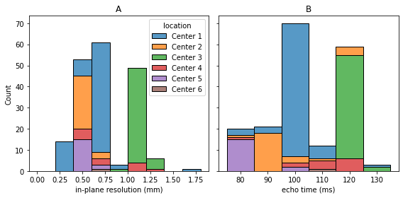
Figure 1: Distribution of acquisition parameters: Even though an imaging protocol was specified for the study; the acquisition parameters vary widely. As example, the in-plane resolution (A) is supposed to be 0.8 mm, but varies between 0.27 mm and 1.64 mm. There are similar variations for the echo time (B), which was supposed to be 110 ms. In general, the data is very heterogeneous, with different parameters used within one center and greater differences between centers.
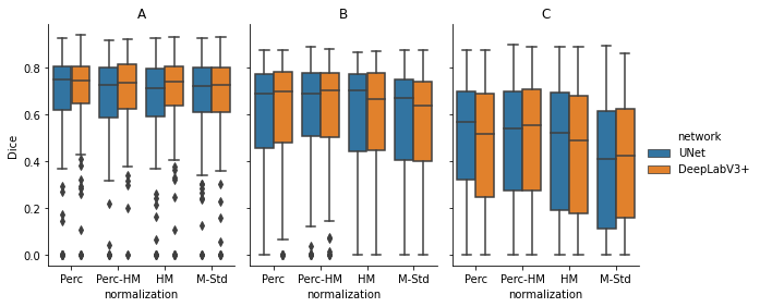
Figure 2: Segmentation Results: In (A), we trained both networks on all images and evaluated them using cross-validation. The results are very similar, with a Dice between 0.71 and 0.74. In (B), we trained on a single center and evaluated on the same center. This results in a performance reduction, probably because of the reduced number of examples. The reduction is even larger for images from different centers, visible in (C). The Dice scores differ significantly depending on the normalization method. The scores vary between 0.41 (M-Std, UNet) and 0.57 (Perc, UNet).
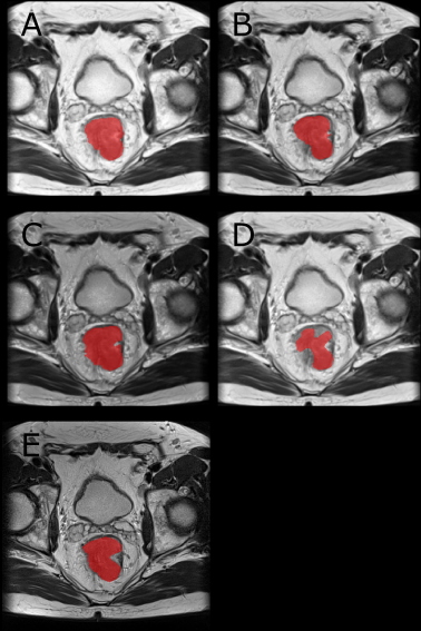
Figure 3: Example Segmentation: A-D are the resulting segmentations when evaluating an image from Center 1 with a network trained on images from Center 3 with the normalizations Perc (A), Perc-HM (B), HM (C) and M-Std (D). The ground truth is visible in E. We trained the networks on multiple graphics cards using the Adam optimizer with a learning rate of 0.001. For the sampling, a ratio sampler was used to reduce the class imbalance. This way, 50 % of slices are centered on a tumor voxel.
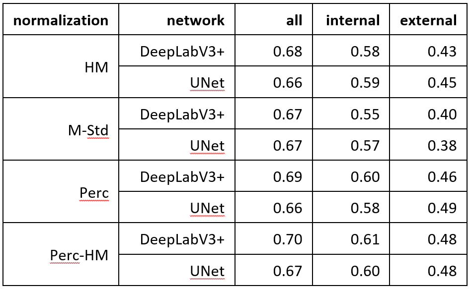
Table 1: Segmentation Results: In this table are the mean Dice scores for different networks and normalization strategies. Column “all” are the Dice scores when training and testing on all available images. Column “internal” are the Dice scores when evaluating on the same center as the training, and in column “external” are the Dice scores when evaluating on all other centers. For the external evaluation, the UNet with Perc normalization performs best and is significantly better than all other methods (p<0.001) besides Perc-HM. For all and internal, no method was significantly better.