Introduction

Head-only asymmetric gradients [1-3] are an approach to build high efficiency, small diameter gradient coils for high-field imaging of the brain, extremities, and infants, but still allow sufficient clinical access to accommodate imaging of human subjects. However, asymmetric gradient coils also introduce additional zeroth-, first-order, and higher-odd-order concomitant fields that need to be compensated for to achieve reliable image quality [4-6]. Salient in the compensation schemes is the knowledge and calibration of the spatial offsets of the asymmetric transverse gradient coils in the z-direction. The Compact 3T (C3T) [2] and MAGNUS [3] head gradients have asymmetric transverse gradient coils, while the z gradient coil is symmetric. Let z_0x and z_0y denote the x and y gradient offsets along the z-direction, for such asymmetric transverse coils, respectively.

To adequately correct for zeroth and first order concomitant gradient terms using pre-emphasis, one must accurately determine the value of these offsets. The offsets can be estimated from the EM analysis of the gradient coil. However, manufacturing tolerances and assembly can introduce errors. The pre-emphasis can be calibrated using trial-and-error methods but a more systematic approach is to use a calibration procedure to determine the z_0x and z_0y offsets, which is described herein.

Methods

The zeroth and first order concomitant fields are given by:
$$B_{error, 0th} \approx \frac{1}{2B_0} \left [ G_x^2 z_{0x}^2 + G_y^2 z_{0y}^2 \right ] \hspace{0.5in} (1) $$
and
$$B_{error,1st} \approx - \frac{G_x G_z z_{0x}}{2 B_0} x - \frac{G_y G_z z_{0y}}{2 B_0} y + \frac{ (G_x^2 z_{0x} + G_y^2 z_{0y})}{B_0}z \hspace{0.5in} (2) $$
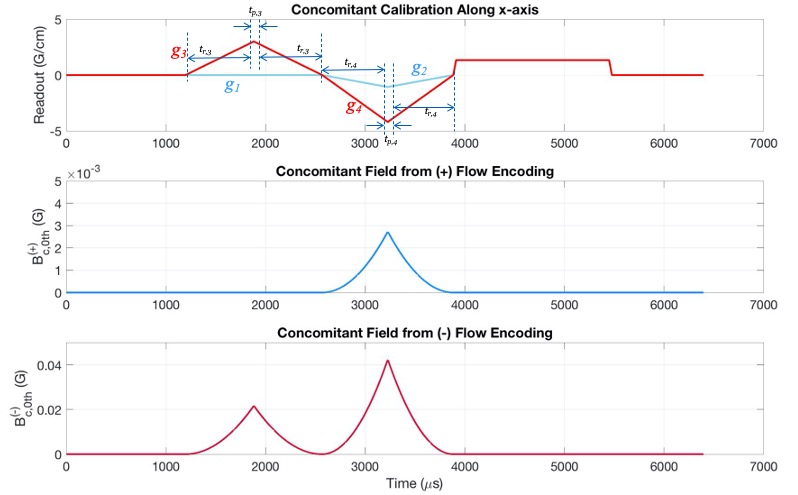
assuming that $$$\alpha$$$ = 0.5 as the z-gradient coil is symmetric. To determine the values of z_0x and z_0y for the Compact 3T (C3T) and MAGNUS gradient coils, a modified phase contrast acquisition sequence with single-sided bipolar gradient waveform was used (Figure 1). The phase difference between the images acquired with the (+) and (-) encoding waveforms yields a non-zero phase in a stationary phantom due to the concomitant fields from the bipolar waveform. As the phase from the (+) or (-) bipolar waveforms are
$$ \phi = \gamma \int_{\tau} B_{error, 0th}(t) dt \hspace{0.5in} (3) $$
the phase difference is
$$ \Delta \phi = \phi^{(+)} - \phi^{(-)} $$
$$ \hspace{3.0in} = \gamma \left[ \int_{\tau} B_{error, 0th}^{(+)} (t) dt - \int_{\tau} B_{error, 0th}^{(-)} (t) dt \right] \hspace{0.5in} (4) $$
By varying the amplitude of the (-) encoding waveform through a range of values, the phase difference measurements is fitted as a function of G_x² or G_y². As g₃ is varied, the gradient offset is determined from the fit to Eq.(4), where a₁ is the coefficient of the quadratic term,
$$z_{0x} = \sqrt{ a_1(\frac{2B_0}{\gamma}) \left( t_{pw,3} + t_{pw,4}\left( \frac{t_{p,3} + t_{r,3}}{t_{p,4} + t_{r,4}} \right)^2 \right)^{-1} } \hspace{0.5in} (5) $$
where t_p,3, t_p,4, t_r,3, t_r,4 are the pulse widths of the bipolar waveforms (Figure 1), and t_pw,i = [t_p,i + (2/3) t_r,i], with i=1,2,3,4 indicating the first and second gradient lobes of the (+) and (-) encoding waveforms. For single-sided encoding, g₁ = 0, and g₂ is simply the gradient lobe acting as the dephasing gradient for the readout gradient.

All experiments were conducted on a C3T (80 mT/m and 700 T/m/s) and two MAGNUS (200 mT/m and 500 T/m/s) systems with 32-channel (NOVA Medical, Wilmington, MA) receiver coils. An oil-filled 14-cm diameter phantom was used for the experiments. To calibrate the offset for the x gradient, an axial 24-cm acquisition with R/L set as the frequency encoding direction was used with a 256 x 256 acquisition matrix with 10-mm slice thickness. “Flow” encoding was along the R/L direction. To calibrate the y gradient offset, “Flow” encoding was along the A/P direction. As a bipolar encoding waveform is used in a stationary phantom, a zero phase is expected. After the phantom settles, any residual phase would be due to eddy currents or concomitant fields. The amplitude of the bipolar encoding (g₃) waveform was varied from $$$\pm$$$40% of the maximum gradient amplitude.

Results

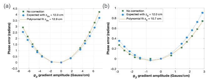
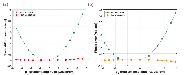
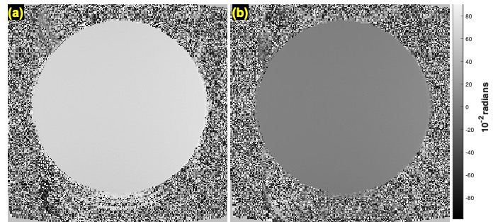
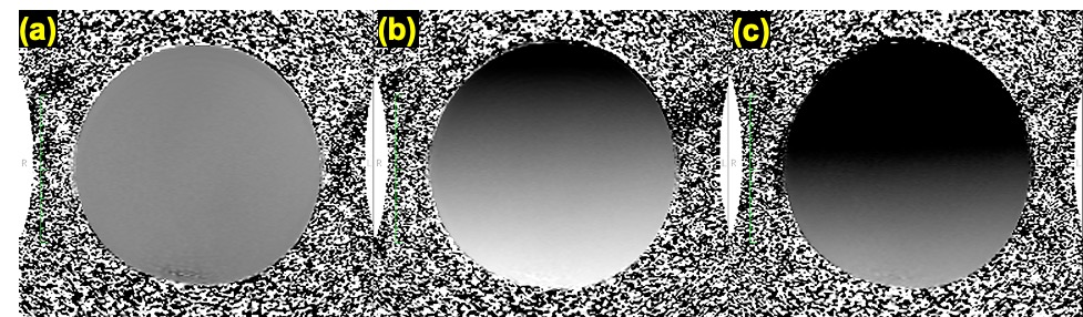
From the EM design of the C3T and MAGNUS gradients, the phase difference or measured phase error as a function of g₃ is shown in Figure 2 for the C3T gradient as well MAGNUS (unit #2). Using the nominal EM value of z_0x of 12 cm in Eq. (4) was slightly off from the measured phase variation in both the C3T and MAGNUS gradients. Using the measured value of z_0x, the zeroth order concomitant frequency correction provided adequate compensation of the concomitant field effects (Figure 3). The measured z_0x offsets were for C3T, 10.7$$$\pm$$$ 0.2 cm, MAGNUS, 12.7$$$\pm$$$0.2 cm and 12.9$$$\pm$$$0.2 cm. The departure of the measured values from the nominal EM values by $$$\pm$$$1 cm was expected due to manufacturing and assembly tolerances, as was the 0.2 cm difference between the two MAGNUS gradients coils.

Discussion

An efficient and simple method to calibrate the concomitant gradient field compensation using a phase difference approach has been described. The gradient offset parameters are used for pre-emphasis compensation for the zeroth and first order concomitant field effects (Figures 4 and 5). This proposed method eliminates a trial-and-error approach to determine the correct scaling parameters for the pre-emphasis correction and accounts for variations in the gradient offsets for asymmetric gradient coils due to manufacturing tolerances.

Acknowledgements

Grant funding: NIH U01EB026976, NIH U01EB024450, and CDMRP W81XWH-16-2-0054