2834

The effects of cutting/zero-filling and linebroadening on quantification of magnetic resonance spectra via maximum-likelihood estimation

Karl Landheer¹ and Christoph Juchem^1,2
¹Biomedical Engineering, Columbia University, New York City, NY, United States, ²Radiology, Columbia University, New York City, NY, United States

Synopsis

It has recently been recommended that typical preprocessing tools, such as linebroadening, zero-filling and apodization (cutting), generally be avoided prior to signal quantification via consensus. To date, little explanation has been provided against these tools which have become commonplace. Here we demonstrate via realistic Monte Carlo simulations that such preprocessing tools may reduce the precision of the extracted parameters and artificially reduce the Cramér-Rao Lower Bounds and provide a theoretical outline for why they should be avoided.

Introduction

Cutting/zero-filling and exponential linebroadening are routine preprocessing tools used prior to quantification of MR spectra as an attempt to tease out more information from the signal. These tools have been implemented in packages such as LCModel¹, TARQUIN², jMRUI³, FID-A⁴, and INSPECTOR⁵. These steps are useful for visualization of spectra but are not recommended prior to quantification^6,7. Here we demonstrate via Monte Carlo simulations that such preprocessing tools might reduce the precision of the extracted parameters and artificially reduce the estimated Cramér-Rao Lower Bounds (CRLBs). We provide a theoretical outline for why these tools should be avoided prior to quantification.

Methods

Spectral shapes were simulated for a TE = 20 ms sLASER⁸ sequence for 18 metabolites and 10 macromolecules which were modeled as broad Lorentzian singlets via MARSS⁹, similar to what has previously been performed^8,11. The macromolecular (MM) signal was modeled as the sum of these 10 macromolecule resonances with measured concentrations and T₂ values¹⁰. The simulated spectral shapes were exponentially linebroadened by $$$\frac{1}{\pi T_2^m}$$$, where $$$T_2^m $$$ is the transverse relaxation constant for the particular metabolite, and all metabolites were broadened by a Gaussian linewidth of 8 Hz² to resemble imperfect B₀ conditions typically encountered in vivo. The broadened spectral shapes were scaled by their respective concentration, and corrected for T₁ and T₂ effects through the solution to the Bloch equation. A synthetic spectrum was used so that ground truth parameters were known, which is not true in any experimental spectrum.

The effect these preprocessing tools had on quantification was assessed by running three different Monte Carlo simulations: 1) no preprocessing, 2) spectra were cut by a factor of two and zero-filled back to the original length (i.e., 2nd half of FID which is almost purely noise was set to zero) and, 3) spectra were linebroadened by a 3 Hz exponential function. A total of 5,000 trials were performed for each case, and spectra differed only by additive white Gaussian noise. For each trial the spectra were quantified using a maximum-likelihood estimator (MLE) in INSPECTOR and CRLBs were calculated¹².

Results and Discussion

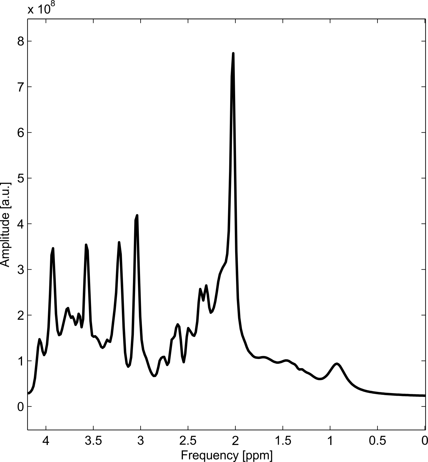
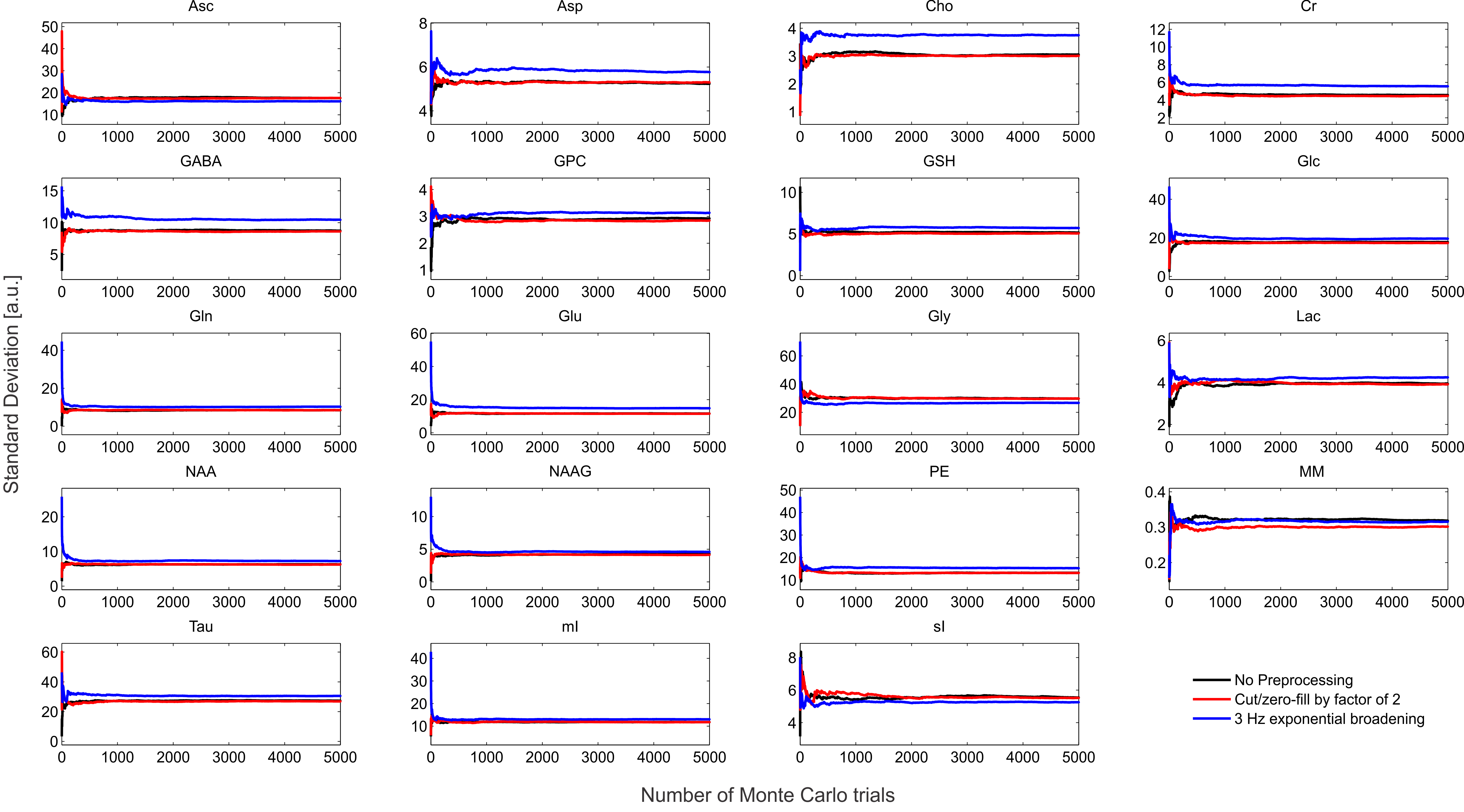
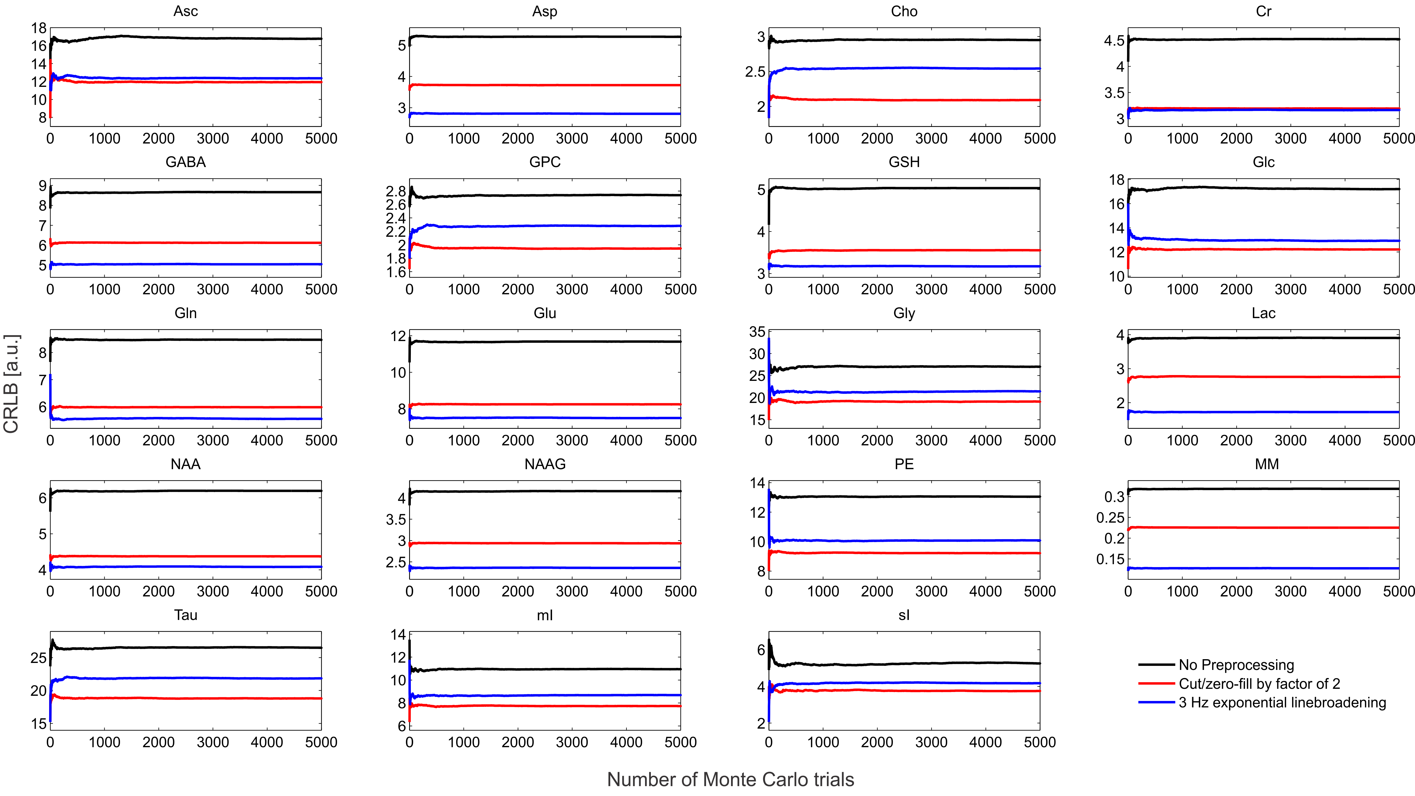
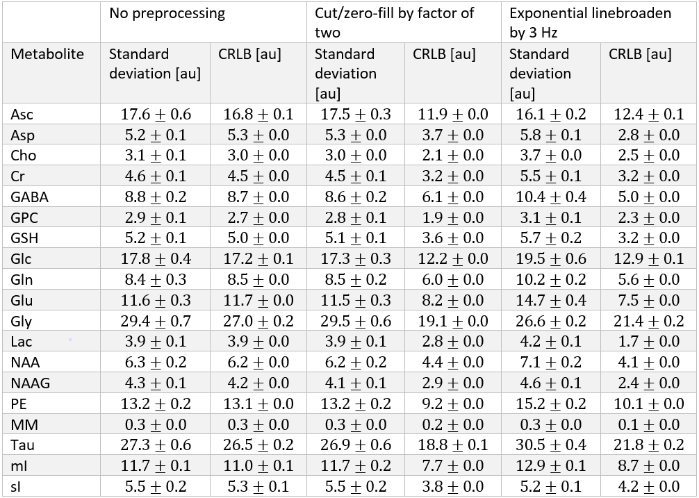
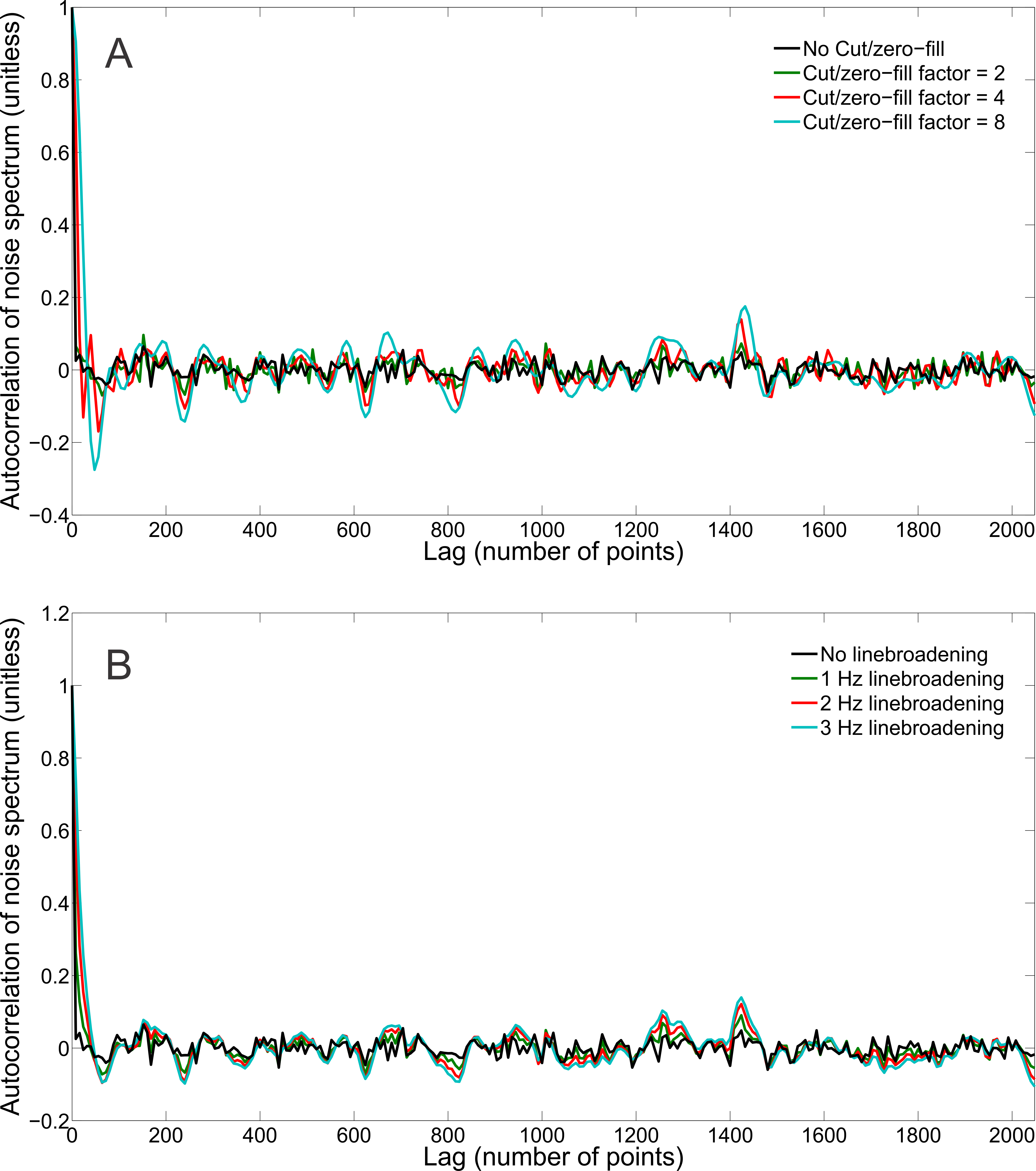
The synthesized spectrum used for the Monte Carlo simulations closely resembles experimental measurements with the same sequence⁸ (Figure 1). Cutting/zero-filling has little effect on measured standard deviations, while the 3 Hz exponential linebroadening noticeably increased the resulting standard deviations (Figure 2). The estimated CRLB values were substantially artificially reduced by both preprocessing steps and no longer become an accurate proxy for standard deviations (Figure 3). In the case where the spectra has been cut/zero-filled by a factor of two the apparent CRLB has been reduced by a factor of $$$\sqrt{2}$$$, whereas the 3 Hz exponential linebroadening reduces the CRLBs by a factor of 1.2 to 2.3 depending on the specific metabolite (Table 1). These results can be understood from the assumptions of the calculation of the CRLBs, namely that the parameters are sampled from a normal distribution due to white Gaussian noise. Cutting/zero-filling the spectrum in the time domain is effectively multiplying it by a step function, hence its effect on the spectrum can be expressed as $$S'(f)=S(f)+S(f)*\left(\frac{1}{2 \pi if}\right), $$
where $$$S'(f)$$$ is the spectrum after preprocessing, $$$S(f)$$$ is the spectrum before preprocessing and $$$*$$$ is the convolution operator. $$$S'(f)$$$ will no longer contain white Gaussian noise, as there is clearly a correlation between spectrally neighboring noise points (Figure 4A). Similarly, the effect of Lorentzian broadening can be expressed as $$ S'(f)=S(f)*\left(\frac{2 \pi LB}{(\pi LB)^2+(2 \pi f)^2}\right)$$
where $$$LB$$$ is the Lorentzian linebroadening width (Hz). Once again this introduces correlation between spectrally neighboring noise points (Figure 4B).

Because CRLBs are a fundamental bound on the standard deviation of parameters irrespective of the method used for estimation¹³, coupled with the results obtained here that the employed maximum-likelihood estimator algorithm effectively attains the CRLBs (Table 1), this demonstrates that the signal is being used nearly as efficiently as possible¹⁴. Thus, signal preprocessing methods are fundamentally unable to yield any substantial information as the information limit has nearly been attained. These preprocessing tools do, however, invalidate the assumptions of the CRLB, specifically that the noise is white and Gaussian, which results in the assumption that the parameters are sampled from a normal probability density function¹⁵, and hence only artificially reduces the CRLBs. Similarly, it has previously been shown that increasing the number of points in the FID which are purely noise has no effect on the CRLB⁷ (and hence quantification precision). This is as expected as the Fisher information matrix (which is proportional to the inverse of the CRLBs) is additive and thus new data points cannot subtract information. Although these points obscure visualization of the spectrum they do not impede the MLE quantification. Note that cutting alone does not violate the assumptions in calculating CRLBs, however cutting data points which contain substantial signal would reduce the precision of the measured parameters.

Conclusions

Cutting/zero-filling and and linebroadening, although useful for data visualization, should not be used prior to quantification as they yield no information while invalidating the assumptions used in the calculation of the CRLBs, causing them to become artificially low. These artificially low CRLBs could potentially result in false positives or statistically under-powered studies.

Acknowledgements

Special thanks to Martin Gajdošík, PhD, and Kelley Swanberg, MSc, for fruitful discussions and input.

References

1. Provencher, S. Estimation of Metabolite Concentrations from Localized in Vivo Proton NMR spectra. Magn Reson Med 30, 672–679 (1993).

2. Wilson, M., Reynolds, G., Kauppinen, R. A., Arvanitis, T. N. & Peet, A. C. A constrained least-squares approach to the automated quantitation of in vivo 1H magnetic resonance spectroscopy data. Magn. Reson. Med. 65, 1–12 (2011).

3. Stefan, D. et al. Quantitation of magnetic resonance spectroscopy signals: The jMRUI software package. Meas. Sci. Technol. 20, 104035 (2009).

4. Simpson, R., Devenyi, G. A., Jezzard, P., Hennessy, T. J. & Near, J. Advanced processing and simulation of MRS data using the FID appliance (FID-A)—An open source, MATLAB-based toolkit. Magn Reson Med 77, 23–33 (2017).

5. Prinsen, H., de Graaf, R. A., Mason, G. F., Pelletier, D. & Juchem, C. Reproducibility measurement of glutathione, GABA, and glutamate: Towards in vivo neurochemical profiling of multiple sclerosis with MR spectroscopy at 7T. J Magn Reson Imag 45, 187–198 (2017).

6. Near, J. et al. Preprocessing, analysis and quantification in single‐voxel magnetic resonance spectroscopy: experts’ consensus recommendations. NMR Biomed. 1–23 (2020). doi:10.1002/nbm.4257

7. Kreis, R. et al. Terminology and concepts for the characterization of in vivo MR spectroscopy methods and MR spectra: Background and experts’ consensus recommendations. NMR Biomed. e4347 (2020). doi:10.1002/nbm.4347

8. Landheer, K., Gajdosik, M. & Juchem, C. Semi-LASER Single-Voxel Spectroscopic Sequence with Minimal Echo Time of 20 ms in the Human Brain at 3 T. NMR Biomed e4324 (2020).

9. Landheer, K., Swanberg, K. M. & Juchem, C. Magnetic resonance Spectrum simulator (MARSS), a novel software package for fast and computationally efficient basis set simulation. NMR Biomed e4129 (2019). doi:10.1002/nbm.4129

10. Landheer, K., Gajdosik, M., Treacy, M. & Juchem, C. Concentration and T2 Relaxation Times of Macromolecules at 3 Tesla. Magn Reson Med 84, 2327–2337 (2020).

11. Bolliger, C. S., Boesch, C. & Kreis, R. On the use of Cramér-Rao minimum variance bounds for the design of magnetic resonance spectroscopy experiments. Neuroimage 83, 1031–40 (2013).

12. Cavassila, S., Deval, S., Huegen, C., Ormondt, D. v & Graveron-Demilly, D. Cramér–Rao bounds: an evaluation tool for quantitation. NMR Biomed 14, 278–283 (2001).

13. Beer, R. & Ormondt, D. Analysis of NMR Data Using Time Domain Fitting Procedures. In-Vivo Magn. Reson. Spectrosc. I Probeheads Radiofreq. Pulses Spectr. Anal. 201–248 (1992). doi:10.1007/978-3-642-45697-8_7

14. Hstadsen, A. On the existence of efficient estimators. IEEE Trans. Signal Process. 48, 3028–3031 (2000).

15. Cavassila, S., Deval, S., Huegen, C., van Ormondt, D. & Graveron-Demilly, D. Cramer-Rao Bound Expressions for Parametric Estimation of Overlapping Peaks: Influence of Prior Knowledge. J Magn Reson 143, 311–320 (2000).

Figures

Figure 1: Synthesized spectrum used for the Monte Carlo simulations. As this spectrum was purely synthesized the true concentrations and the model which perfectly represents the data is known a priori, hence standard deviations (not standard errors) can be calculated.

Figure 2: Standard deviation of fitted amplitude for no preprocessing (black), Cut/zero-fill by factor of two (red) and 3 Hz exponential line broaden (blue) across the 5,000 Monte Carlo simulations for the 18 metabolites and macromolecules (MM). Exponential linebroadening increases the standard deviation (for most metabolites), while cut/zero-fill has little effect on the precision.

Figure 3: Estimated CRLBs for amplitude for no preprocessing (black), Cut/zero-fill by factor of two (red) and 3 Hz exponential line broaden (blue) across the 5,000 Monte Carlo simulations for the 18 metabolites and macromolecules (MM). The preprocessing steps artificially reduce the estimated CRLB values. Note that these CRLBs are in the same units of amplitude and its standard deviation (i.e., au), it is not relative CRLBs (in %) as is typically presented in MRS.

Table 1: The standard deviation and CRLB for the 18 measured metabolites and macromolecules (MM) across the three different pipelines. Note that for no preprocessing the CRLB is an excellent proxy for standard deviation for all metabolites, while there is an artificial reduction of CRLBs for the two preprocessing steps. Furthermore, the exponential line broadening results in a reduction in precision on most metabolites. Note that these CRLBs are in the same units of standard deviation (i.e., au), it is not relative CRLBs (%) as is typically presented in MRS.

Figure 4: The effect cutting/zero-filling, A, and exponential linebroadening, B, has on the autocorrelation function of a simulated white Gaussian noise spectrum. In both cases as the effect of the processing steps is increased the autocorrelation of the noise spectrum deviates further from its assumed shape of $$$\delta(f)$$$. Cut/zero-fill factor = 2/4/8 means that the entire time domain signal except for the first half/quarter/eighth has been artificially set to zero.

Proc. Intl. Soc. Mag. Reson. Med. 29 (2021)

2834