2100
Simulation of Flowing Spins in MRI using the Lattice Boltzmann Method1Institute for Diagnostic and Interventional Radiology, (UMG) University Medical Center Göttingen, Göttingen, Germany, 2Biomedical NMR, Max Planck Institute for Biophysical Chemistry, Göttingen, Germany, 3Max Planck Institute for Dynamics and Self-Organization, Göttingen, Germany, 4DZHK (German Centre for Cardiovascular Research), Göttingen, Germany
Synopsis
The lattice Boltzmann method (LBM) is a versatile numerical technique for simulating complex fluid dynamical systems and beyond. Here, we first describe an extension of the LBM to flow systems in external magnetic fields. The model is verified numerically with several benchmarks and shown to correctly predict signal changes caused by in-flow effects in a simple flow experiment.
Introduction and Purpose
Simulation of flow in MRI is of high interest for the investigation of flow dynamics and understanding of imaging artifacts. At present, most related simulations use conventional techniques from computational fluid dynamics to resolve the Navier-Stokes equation first, and second, use the Bloch equations to simulate particles flowing along streamlines of the flow field [4] thus there were two coupled techniques in the previous [5]. These techniques are fundamentally limited, e.g. they cannot model fully coupled flow and diffusion effects in MRI. In this work, we extend the lattice Boltzmann method (LBM) [1] by modeling the internal spin degree of freedom as part of a joint velocity-spin-distribution. The proposed technique recovers the Navier-Stokes equation and Bloch-Torrey equation.Theory
Velocity-Spin DistributionIn the conventional LBM, the distribution function $$$f(\vec{r}, t)$$$ of a fluid particle is discretized in physical space, time, and velocity space $$$f_i(\vec{r}, t) = f(\vec{r}, \vec{c}_i, t)$$$, with $$$\vec{r}$$$ the location on a spatial grid, $$$t$$$ the time step, and $$$i$$$ the index of the discretized velocity vectors $$$\vec{c}_i$$$. The statistical state of the internal spin degree of freedom of an ensemble of spin 1/2 particles, as the H$$$^1$$$ nucleus, is described by the quantum mechanical density operator $$$D$$$, which can be decomposed into Pauli matrices according to
$$ D = \frac{1}{2}\left( \sigma_0 + \vec a \cdot \vec \sigma \right) = \frac{1}{2}\left( \sigma_0 + a_x \sigma_x + a_y \sigma_y + a_z \sigma_z \right),$$
where $$$\vec \sigma$$$ is the vector of the three Pauli matrices $$$\sigma_x, \sigma_y, \sigma_z$$$, and $$$\sigma_0$$$ the identity matrix, and $$$\vec a$$$ the Bloch vector [3]. The macroscopic magnetization is related to the quantum mechanical expectation value of the spin which is given by the density matrix multiplied with the spin observable: $$$\gamma \frac{\hbar}{2} {\bf Tr} D \vec{\sigma}$$$. We propose a model of flowing particles with spin 1/2 using a matrix-valued semi-classical velocity-spin distribution $$$D(\vec r, t)$$$ and discretize it by
$$D_i(\vec r, t) := \frac{1}{2} \sum_j f_{i,j}(\vec r, t) \sigma_j, $$
where $$$j$$$ denotes the polarization direction $$${0,x,y,z}$$$. The positivity of the coefficient $$$f_i$$$ in the classical LBM corresponds to positive definiteness of the matrix $$$D_i$$$. Summing over all velocity directions recovers the density $$$\rho$$$, the bulk velocity $$$\vec u$$$, and the components of the macroscopic magnetization $$$\vec M$$$ at each lattice node according to
$$\rho = \sum_i f_{i,0}, \qquad \rho \vec u = \sum_i f_{i,0} \vec c_i, \quad \text{ and } \quad M_j = \sum_i f_{i,j} \text{ .}$$
Incorporation of the Velocity-Spin Distribution in LBM
The LBM simulates the discretized Boltzmann equation [1] in a streaming and collision step. The streaming step works on each $$$j$$$ independently and transports each component $$$f_{i,j}$$$ to the next grid point in the direction $$$\vec c_i$$$. The BGK collision step is
$$ f'_{i,j'} \leftarrow \sum_j B_{j',j} \left( f_{i,j} - \frac{f_{i,j} - f^{eq}_{i,j}}{\tau} \right), $$
with the relaxation time $$$\tau$$$, post-collision distribution $$$f'_{i,j}$$$ and equilibrium function $$$f^{eq}_{i,j}$$$. Here, we assume a common equilibrium distribution for the velocities defined by $$$\rho$$$ and $$$\vec u$$$ and independent from the magnetization as in the standard LBM. The matrix $$$B_{j,j'}$$$ implements a step of the time-discretized Bloch equations, modelling relaxation and the effect of all external fields.
Methods
Numerical ValidationSeveral canonical flows, e.g. the Pouiseuille flow, backward facing step flow and Karman vortex street, were considered. Numerical results with the proposed model agree well with the benchmarks. Furthermore, we showed that for zero flow the magnetization recovers the Ernst equation, i.e. steady-state magnetization [2] for a spoiled FLASH sequence. Finally, the agreement with the Bloch-Torrey equation was verified numerically.
Experimental Setup
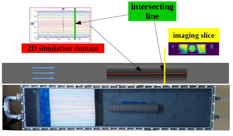
Developing laminar pipe flow with different flow rates, controlled by the pump-level, was considered. To verify the prediction of the signal change caused by the in-flow of spins, flow through a cross-sectional slice was measured experimentally with a phase-contrast FLASH sequence. Slice thickness and flip angle were varied. We then simulated the flow and magnetization of such an experiment in a plane adapting the velocity in the center to the one determined by phase-contrast MRI. In the intersection line of the measured slice and the simulated plane, the signal intensities were compared between experiment and simulation (Fig. 1).
Results
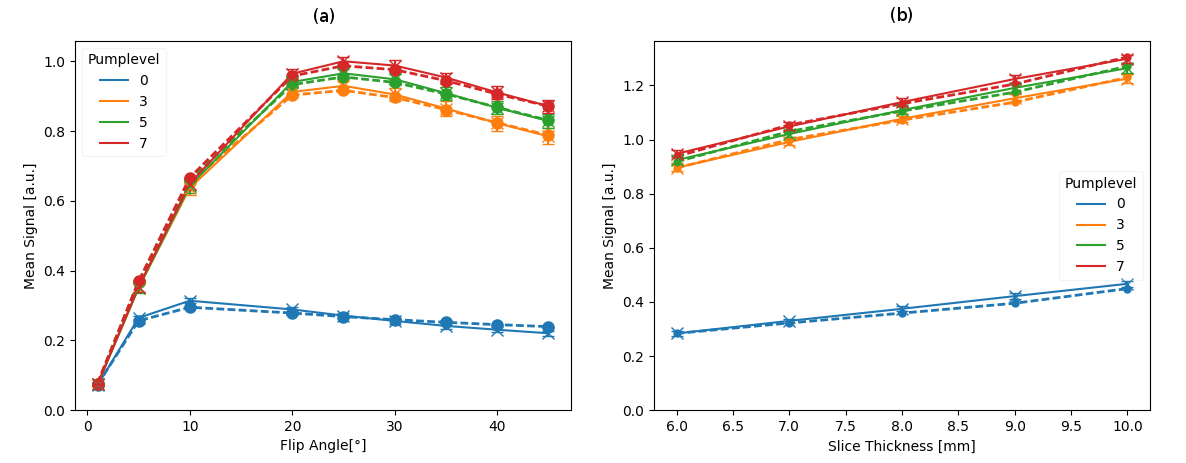
The global relative error for the Pouiseuille flow and steady-state magnetization are less than 1%. Furthermore, the length and vorticity of the vortices in the Karman vortex street and pipe expansion agree with literature.Fig. 2 shows the measured signal and velocity profiles for varying pump-levels in comparison to the numerical ones from simulations. Flat profiles in the center imply that the flows were developing. Considering the discrepancy in the flow profiles in the 3D experiment and the 2D simulation, analysis is restricted to a region of homogenous flow in the center.
Fig. 3 depicts the numerical and experimental mean signal levels for the region marked gray in Fig. 2 for varying flip angle and slice thickness.
Discussion and Outlook
In this work, we developed a model for simulating flow phenomena in MRI using the LBM to simulate both spin physics and fluid dynamics in a unified framework. In an experimental test related to in-flow effects, numerical and experimental results agree with only small deviations.Acknowledgements
Supported by the DZHK (German Centre for Cardiovascular Research).References
[1] Krüger T., Halim K., The Lattice Boltzmann Method, Springer-Verlag, 2017.
[2] Liang Z. P., Lauterbur P. C., Principles of Magnetic Resonance Imaging: A Signal Processing Perspective, IEEE Press Series on Biomedical Engineering. Wiley, 1999.
[3] Blum K., Density Matrix Theory and Applications, Plenum Press, 1981.
[4] Puiseux T., Sewonu A., Moreno R., Mendez S., and Nicoud F., Numerical simulation of 4D Flow MRI. ISMRM Virtual Conference & Exhibition 2020, In Proc. Intl. Soc. Mag. Reson. Med. 28; 1042, 2020.
[5] Jurczuk K., Kretowski M., Bellanger J., Eliat P., Saint-Jalmes H., Bézy-Wendling J., Computational modeling of MR flow imaging by the lattice Boltzmann method and Bloch equation. In Magnetic Resonance Imaging Vol 31; 7, 2013.
Figures