1996
Accelerate Magnetic Resonance Spectroscopy with Deep Low Rank Hankel Matrix1Department of Electronic Science, National Institute for Data Science in Health and Medicine, Xiamen University, Xiamen, China, 2School of Computer and Information Engineering, Xiamen University of Technology, Xiamen, China
Synopsis
Nuclear Magnetic Resonance (NMR) spectroscopy is regarded as an important tool in bio-engineering while often suffers from its time-consuming acquisition. Non-Uniformly Sampling (NUS) method can speed up the acquisition, but the missing FID signals need to be reconstructed with proper method.. In this work, we proposed a deep learning reconstruction method based on unrolling the iterative process of a state-of-the-art model-based low rank Hankel matrix method. Experimental results show that the proposed method provides a better approximation of low rank and preserves the low-intensity signals much better.
Purpose
NMR spectroscopy serves as an indispensable biophysical tool in modern chemistry and life science. To accelerate the FID signals acquisition, different methods have been established to reconstruct the NUS NMR spectroscopy, including model-based iterative algorithms1-6 and deep learning method7, 8. The former require different kinds of prior assumption which may not well utilize the best features, while the latter is lack of interpretability. As a state-of-the-art iterative algorithm, Low Rank Hankel Matrix Factorization (LRHMF)5, 6 utilizes the low rank property of the Hankel matrix generated from fully sampled FID as a constraint. In this work, we unfold the LRHMF algorithm to a so-called Deep Hankel Matrix Factorization network (DHMF). Experiments show that the proposed method provides a better approximation of low rank property, which is easier to interpret than existing deep learning-based method. DHMF also achieves lower reconstruction error than the compared state-of-the-art methods and preserves the low-intensity signals much better.Methods
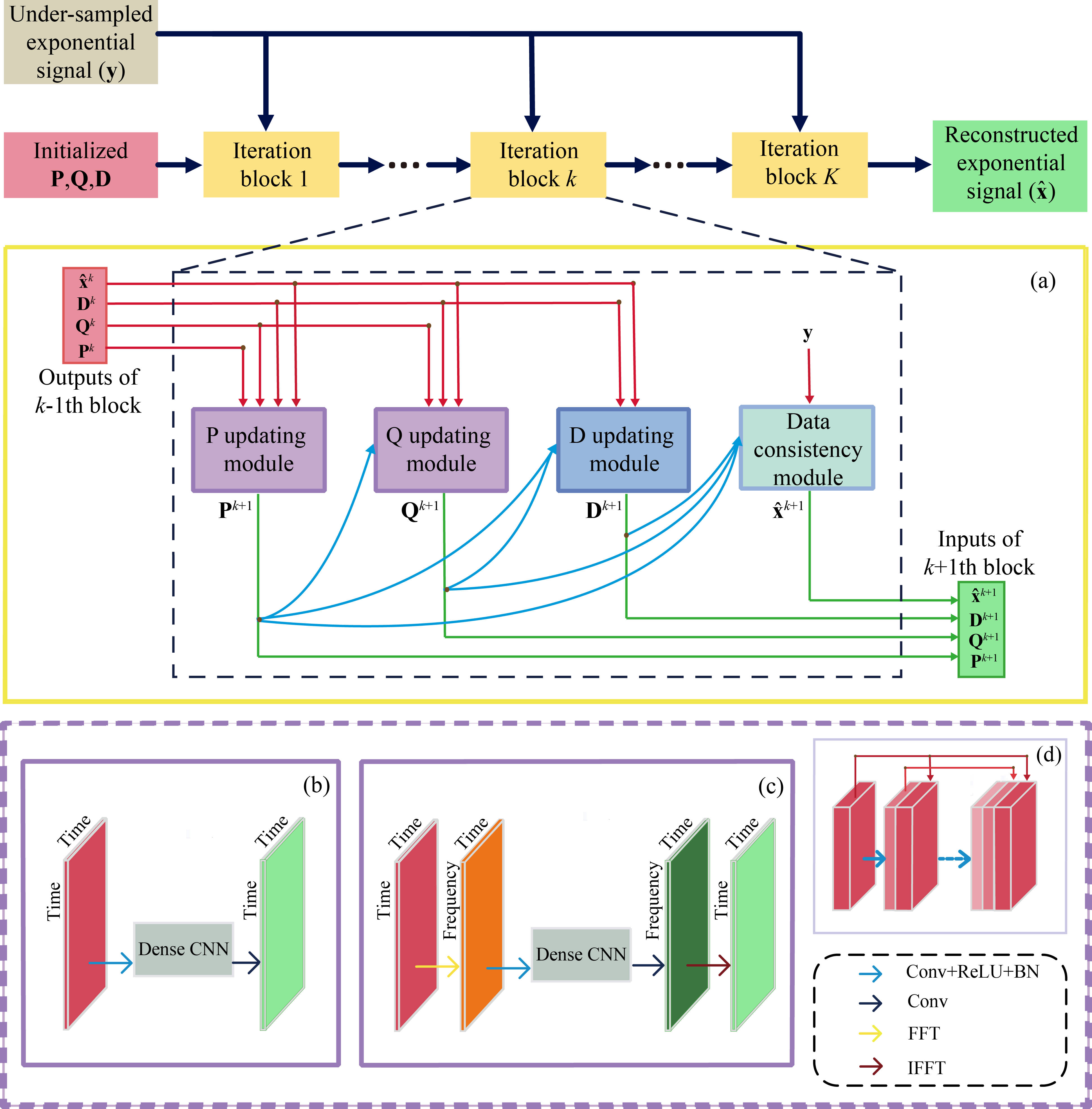
Considering the success that Deep Learning NMR (DLNMR)7 can be solely trained by synthetic FID, we generate the training dataset, i.e. fully sampled FID $$$\mathbf{x}$$$, as the superposition of numbers of exponential functions. The corresponding spectrum can be denoted as $$$\mathbf{Fx}$$$, where $$$\mathbf{F}$$$ is the Fourier transform, and the NUS FID satisfies $$$\mathbf{y}\text{=}\mathbf{Ux}$$$, where $$$\mathbf{U}$$$ denotes the NUS operator.Inspired by LRHMF5, 6 to obtain reconstructed FID $$$\mathbf{\hat{x}}$$$, we unfold its iterative process into three updating modules $$$\mathbf{P},\mathbf{Q},\mathbf{D}$$$ and one data consistency module (Fig.1(a)), corresponding to the updating of four intermediate variables in the iterative process. The initial variables that input the neural network are calculated by factorizing $$$\mathsf{\mathcal{R}}\mathbf{y}\text{=}\mathbf{PQ}_{{}}^{H}$$$, where $$$\mathsf{\mathcal{R}}$$$ is the Hankel operator which turns a vector to a Hankel matrix, while $$$\mathbf{D}$$$ is initialized by zero matrix.
The updating modules of $$$\mathbf{P},\mathbf{Q}$$$ in the k-th (k=1, 2…, K) iteration block can be modified as:
$$\begin{align} & {{\mathbf{P}}^{k+1}}={{\mathsf{\mathcal{P}}}^{k}}((\mathsf{\mathcal{R}}{{{\mathbf{\hat{x}}}}^{k}}+{{\mathbf{D}}^{k}}){{\mathbf{Q}}^{k}},{{\mathbf{Q}}^{k}},{{\mathbf{P}}^{k}}) \\ & {{\mathbf{Q}}^{k+1}}={{\mathsf{\mathcal{Q}}}^{k}}({{(\mathsf{\mathcal{R}}{{{\mathbf{\hat{x}}}}^{k}}+{{\mathbf{D}}^{k}})}^{H}}{{\mathbf{P}}^{k+1}},{{\mathbf{P}}^{k+1}},{{\mathbf{Q}}^{k}}) \\ \end{align},\ (1) $$
where the variables $$$ (\mathsf{\mathcal{R}}{{\mathbf{\hat{x}}}^{k}}+{{\mathbf{D}}^{k}}){{\mathbf{Q}}^{k}}$$$, $$${{\mathbf{Q}}^{k}}$$$, $$${{\mathbf{P}}^{k}}$$$ are concatenated (Eq. (1)) to be the input of updating module $$$\mathbf{P}$$$ (Fig.1(b)), which is an 8-layers densely connected convolutional neural network9. This module learns a mapping $$${{\mathsf{\mathcal{P}}}^{k}}$$$ to yield the updated variable $$${{\mathbf{P}}^{k+1}}$$$ and updating module $$$\mathbf{Q}$$$ is designed similarly for the updated variable $$${{\mathbf{Q}}^{k+1}}$$$ . Since convolution in frequency domain equals to multiplication in whole time domain, which may better utilize the global information, fast Fourier Transform (FFT) and inverse FFT are utilized on the columns of input and output of $$$\mathbf{P}$$$, $$$\mathbf{Q}$$$ updating module (Fig.1(c)), which means the convolution is performed in frequency domain.
The updating module $$$\mathbf{D}$$$ is then calculated by:
$${{\mathbf{D}}^{k+1}}={{\mathbf{D}}^{k}}+\tau (\mathsf{\mathcal{R}}{{\mathbf{\hat{x}}}^{k}}-{{\mathbf{P}}^{k+1}}{{({{\mathbf{Q}}^{k+1}})}^{H}}),\ (2) $$
where $$$\tau $$$ is set as a constant.
The data consistency module is designed to ensure that reconstructed time-domain signal is aligned to the sampled FID $$$\mathbf{y}$$$ . Given the updated variables $$${{\mathbf{P}}^{k+1}}$$$, $$${{\mathbf{Q}}^{k+1}}$$$ and $$${{\mathbf{D}}^{k+1}}$$$, the reconstructed spectrum is modified as:
$${{\mathbf{\hat{x}}}^{k+1}}=\mathsf{\mathcal{S}}(\mathbf{y},{{\mathsf{\mathcal{R}}}^{*}}({{\mathbf{P}}^{k+1}}{{({{\mathbf{Q}}^{k+1}})}^{H}}-{{\mathbf{D}}^{k+1}})),\ (3)$$
where $$$\mathsf{\mathcal{S}}$$$ denotes the data consistency operator, indicating that the signal at the location of sampled FID should maintain a trade-off between the sampled and reconstructed FID.
The overall loss function in our implementation contains two parts, which are the mean square error between reconstructed $$${{\mathbf{\hat{x}}}^{k+1}}$$$ and fully sampled FID $$$\mathbf{x}$$$, matrix $$${{\mathbf{P}}^{k+1}}{{({{\mathbf{Q}}^{k+1}})}^{H}}$$$ and $$$\mathsf{\mathcal{R}}\mathbf{x}$$$ in all K blocks.
Results
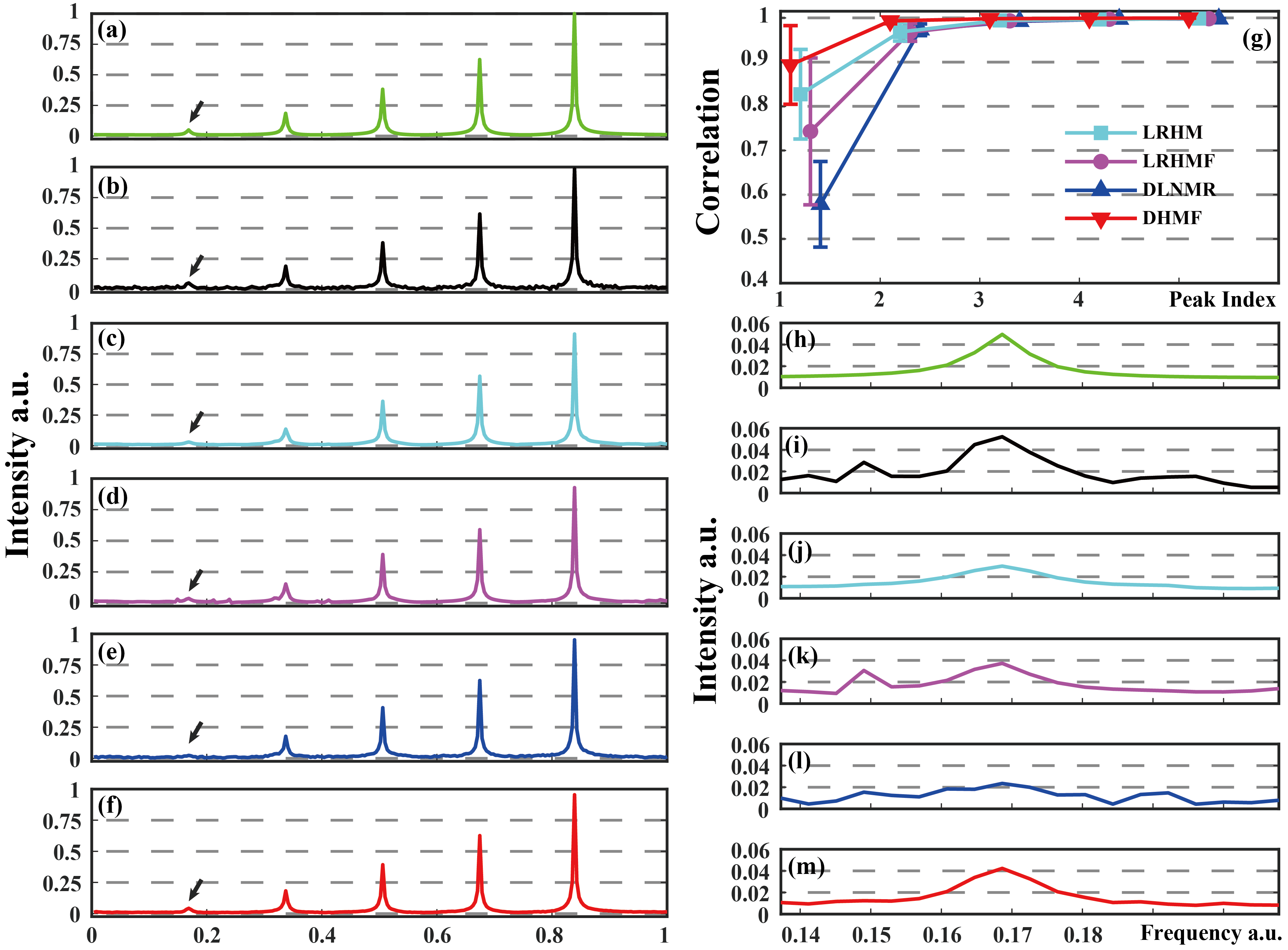
Three state-of-the-art NMR spectroscopy reconstruction approaches are compared, including Low Rank Hankel Matrix (LRHM)1, LRHMF5, and DLNMR7. Both LRHM and LRHMF are model-based iterative algorithms, while DLNMR is a deep learning method.The analysis of intermediate reconstructed results of synthetic FID (Fig. 2) indicate that, in each block (Figs. 2(h)-(l)), the DHMF provides a much better approximation of singular values than DLNMR. At the last block (Fig. 2(l)), DHMF provides very close singular values, although they are not exactly the same, to that of the fully sampled FID. These observations imply that the proposed method provides a better approximation of low rank and better interpretation of the reconstruction in the network. Synthetic FID (Fig. 3) consists of five peaks with at most 20 times spectral intensity. Peak intensity correlation (Fig. 3(g)) demonstrates that DHMF provides the most consistent spectral peak shape and intensity to the fully sampled peak. DLNMR hardly retrieves the weakest peaks while both LRHM and LRHMF introduce pseudo peak around the ground-truth weak peak.
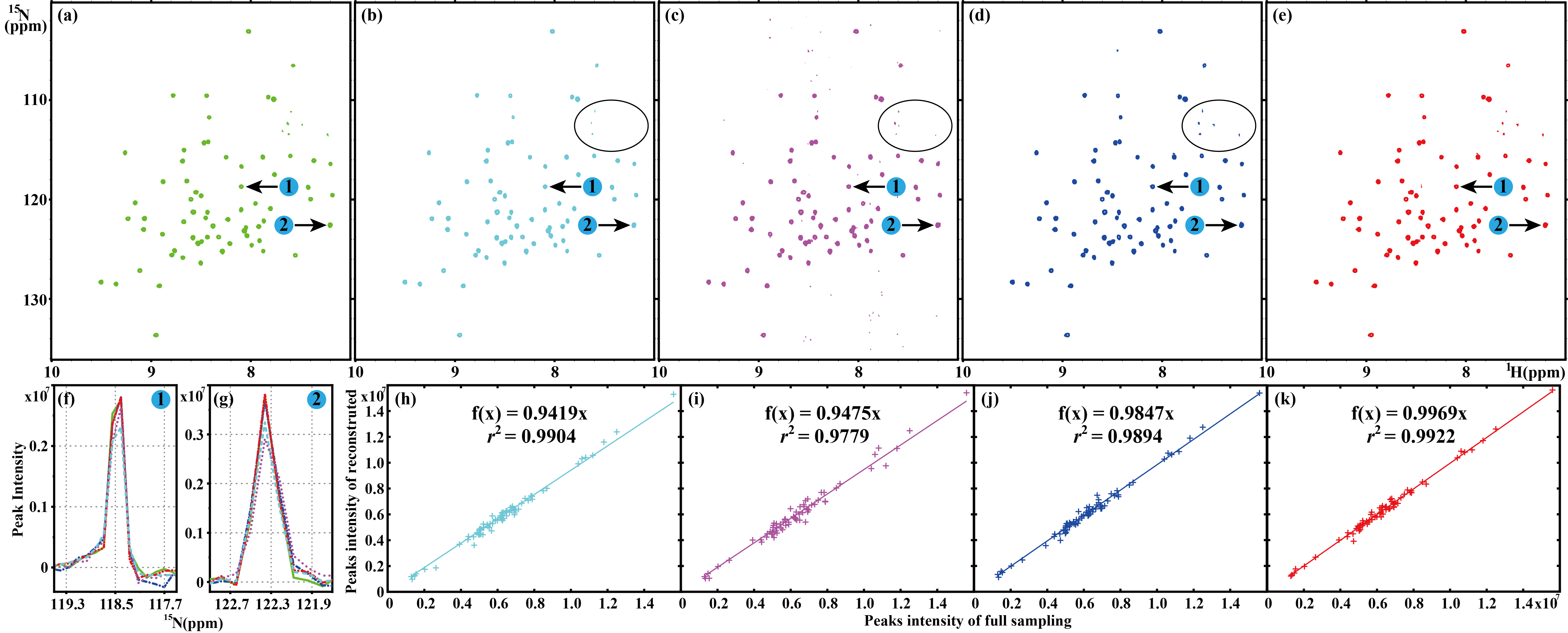
For realistic NMR spectra, one 2D 1H-15N TROSY spectrum of ubiquitin are reconstructed (Fig. 4). DHMF obtains a faithful reconstruction while LRHM underestimates the intensity of peaks, and LRHMF introduces pseudo peaks. Besides, all the compared methods lose weak peaks marked in the black circle, but DHMF does not. DHMF also achieves the highest correlation r among all methods. Therefore, the proposed method provides the most faithful reconstruction for the realistic NMR spectra.
Conclusion
In this work, we propose a new deep learning neural network called DHMF by unrolling the model-based matrix factorization for NMR spectrum undersampled reconstruction. Experimental results on synthetic FID and realistic biological spectra demonstrate that the DHMF outperforms state-of-the-art model-based and deep learning-based methods on preserving low-intensity signals and obtains more faithful reconstruction.Acknowledgements
This work was supported in part by the National Natural Science Foundation of China (61971361, 61871341, 61811530021 and U1632274), the National Key R&D Program of China (2017YFC0108703), the Natural Science Foundation of Fujian Province of China (2018J06018), the Fundamental Research Funds for the Central Universities (20720180056 and 20720200065), and Xiamen University Nanqiang Outstanding Talents Program.
The correspondence should be sent to Dr. Xiaobo Qu (Email: quxiaobo@xmu.edu.cn).
References
[1] Qu X, Mayzel M, Cai J-F, et al. Accelerated NMR spectroscopy with low-rank reconstruction. Angew. Chem.-Int. Edit. 2015;54(3):852-854.
[2] Nguyen H M, Peng X, Do M N, et al. Denoising MR spectroscopic imaging data with low-rank approximations. IEEE Trans. Biomed. Eng. 2013;60(1):78-89.
[3] Ying J, Lu H, Wei Q, et al. Hankel matrix nuclear norm regularized tensor completion for N-dimensional exponential signals. IEEE Trans. Signal Process. 2017;65(14):3702-3717.
[4] Ying J, Cai J-F, Guo D, et al. Vandermonde factorization of Hankel matrix for complex exponential signal recovery—application in fast NMR spectroscopy. IEEE Trans. Signal Process. 2018;66(21):5520-5533.
[5] Guo D, Lu H and Qu X. A fast low rank Hankel matrix factorization reconstruction method for non-uniformly sampled magnetic resonance spectroscopy. IEEE Access 2017;516033-16039.
[6] Lu H, Zhang X, Qiu T, et al. Low rank enhanced matrix recovery of hybrid time and frequency data in fast magnetic resonance spectroscopy. IEEE Trans. Biomed. Eng. 2018;65(4):809-820.
[7] Qu X, Huang Y, Lu H, et al. Accelerated nuclear magnetic resonance spectroscopy with deep learning. Angew. Chem.-Int. Edit. 2020;59(26):10297-10300.
[8] Chen D, Wang Z, Guo D, et al. Review and prospect: Deep learning in nuclear magnetic resonance spectroscopy. Chem.-Eur. J. 2020;2610391-10401.
[9] Huang G, Liu Z, Van Der Maaten L, et al. Densely connected convolutional networks, in Proc. IEEE Comput. Soc. Conf. Comput. Vision Pattern Recognit., 2017;4700-4708
Figures