1964

Using Untrained Convolutional Neural Networks to Accelerate MRI in 2D and 3D

Dave Van Veen^1,2, Arjun Desai¹, Reinhard Heckel^3,4, and Akshay S. Chaudhari¹
¹Stanford University, Stanford, CA, United States, ²University of Texas at Austin, Austin, TX, United States, ³Rice University, Houston, TX, United States, ⁴Technical University of Munich, Munich, Germany

Synopsis

We investigate untrained convolutional neural networks for accelerating both 2D and 3D MRI scans of the knee. Machine learning has demonstrated great potential to accelerate scans while maintaining high quality reconstructions. However, these methods are often trained over a large number of fully-sampled scans, which are difficult to acquire. Here we demonstrate MRI acceleration with untrained networks, achieving similar performance to a trained baseline. Further, we use undersampled k-space measurements as regularization priors to increase the robustness of untrained methods.

Introduction

Supervised machine learning (ML) methods have demonstrated great potential for accelerated MRI by reconstructing images from under-sampled k-space measurements^1-4. However, these methods typically require supervised end-to-end training using large, fully-sampled k-space datasets. Additionally supervised ML often has difficulty generalizing reconstructions across different anatomies, scanner types, and acceleration factors. These fundamental limitations motivate the use of untrained methods, which use gradient descent to optimize network weights given only a single set of undersampled measurements. Untrained methods have shown promise for inverse problems such as denoising and compressed sensing but have not been thoroughly investigated for MRI acceleration^5-9. Here, we demonstrate the ability of untrained networks to accelerate 2D and 3D MRI scans, achieving comparable results to state-of-the-art supervised baseline. Further, we use undersampled k-space measurements as regularization priors to increase the robustness of untrained methods.

Methods

Formulation
Let $$$x$$$ be the MR image we are trying to reconstruct and $$$y$$$ be the fully-sampled k-space, i.e. $$$y=Fx$$$ where $$$F$$$ denotes the Fourier transform. Given the masked k-space $$$\tilde{y}=My$$$, our goal is to generate $$$\hat{x}$$$ close to $$$x$$$ using an untrained network $$$G(z;w)$$$, which maps some random, fixed input seed $$$z\in\mathcal{R}^k$$$ to the reconstruction $$$\hat{x}$$$. We randomly initialize the weights $$$w\in\mathcal{R}^d$$$ and let $$$w^\ast$$$ be the weights obtained by applying a first order gradient method to the loss:
$$\mathcal L(w) =\sum_{i=1}^{n_c}\| \tilde{y}_i-MFG_i(z;w)\|^2 + \lambda R(w).$$
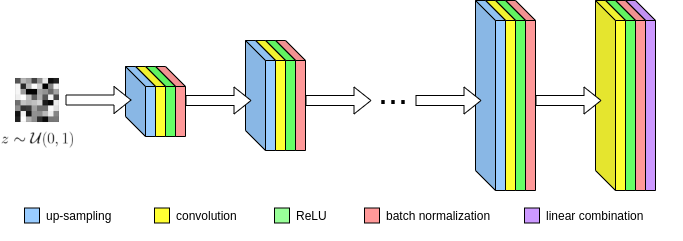
Here, $$$\tilde{y}_i$$$ corresponds to masked k-space measurements from the $$$i^{\text{th}}$$$ of $$$n_c$$$ total coils. Once the optimal weights $$$w^*$$$ are obtained, we can now estimate the MR image $$$\hat{x}$$$ by combining coil reconstructions $$$G_i(z;w^*)$$$ using the SENSE method. Lastly we enforce data consistency regularization between the network's feature maps and the acquired k-space. Our convolutional network $$$G$$$ is based upon the architecture of ConvDecoder⁸, where each layer is comprised of nearest neighbor up-sampling, 3x3 convolutions, ReLU, and batch normalization (Figure 1). The final layer excludes up-sampling and linearly combines network channels into the output image. Due to the progressive upsampling operations, every subsequent layer is larger than the last. Hence linear combinations of intermediate layers represent downsampled versions of the full-sized network output.

Building upon this intuition, we introduce the feature map regularization term $$$R(w)=\sum_{j=1}^{L}\|D^j\tilde{y}-MFG^j(z;w)\|^2$$$ with layer index $$$j=1..L$$$, where $$$G^j(z;w)$$$ refers to the output of the $$$j^{\text{th}}$$$ layer, and $$$D_j$$$ is an operator which downsamples k-space measurements to the appropriate size of that layer. This term encourages fidelity between the network's intermediate representations and the acquired k-space measurements.

Datasets
We evaluate our method with 4x and 8x undersampling on both 2D fast-spin-echo fastMRI scans¹⁰ and clinical 3D quantitative double-echo in steady-state (qDESS) scans¹¹. The fastMRI scans are undersampled using a 1D variable-density mask in $$$k_y$$$, while qDESS scans are undersampled using a 2D variable-density Poisson disc mask in $$$k_y$$$ and $$$k_z$$$. For both datasets we evaluate our method on the central slice of each volume. Our final test set is 73 sagittal slices for fastMRI and 32 axial slices for qDESS, each from unique subjects.

Evaluation
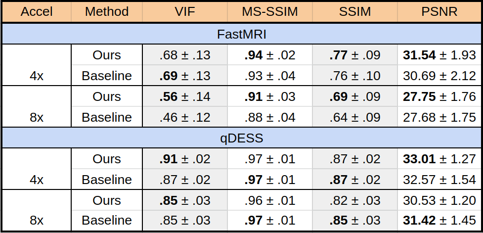
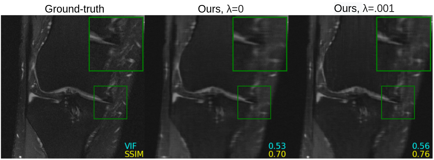
We evaluate our untrained method both without and with feature map regularization, i.e. $$$\lambda=0$$$ and $$$\lambda=.001$$$, respectively, running for 10,000 iterations. As the baseline we compare with a supervised, state-of-the-art, unrolled network architecture containing eight residual blocks, which has shown promise for complex-valued image recovery¹². These networks were trained across 40 fastMRI scans (1400 slices) and 20 qDESS scans (3200 slices), respectively. To measure image reconstruction quality, we use visual information fidelity (VIF), multi-scale SSIM (MS-SSIM), SSIM, and PSNR. Amongst these metrics, VIF has been shown to be the most clinically relevant for diagnostic image quality¹³.

Results and Discussion

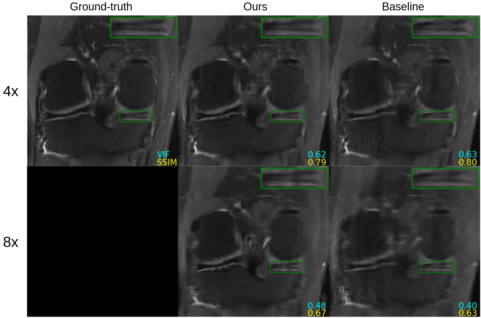
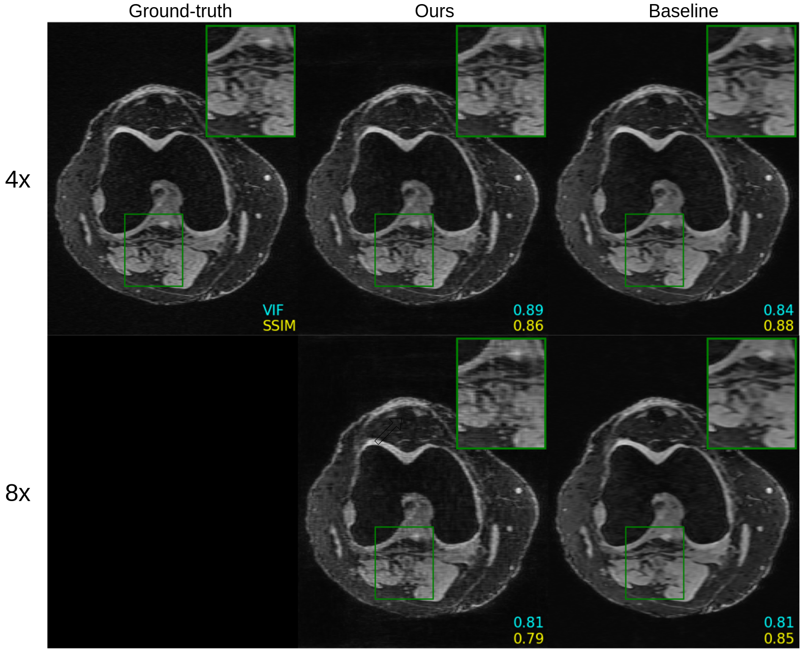
Figure 2 shows quantitative results for our untrained method without feature map regularization, i.e. $$$\lambda=0$$$. Our untrained reconstructions maintain comparable image quality as the supervised baselines for both the fastMRI (Figure 3) and qDESS scans (Figure 4).

Quantitatively the feature map regularization technique results in an improvement on 81% of slices, but the margin is small: typically less than 1%. However for slices with poorer reconstruction when $$$\lambda=0$$$, the improvement can be considerable (example in Figure 5). Such a regularization may mitigate against hallucinations of unwanted features during undersampled MRI reconstruction.

Conclusion

We demonstrate that untrained methods obtain similar performance to supervised baselines for reconstructing 2D and 3D MRI scans across various acceleration factors. Further, we propose a regularization technique which encourages fidelity between the network feature maps and acquired measurements for improving the robustness of MRI reconstruction.

Acknowledgements

We would like to acknowledge our funding sources: National Institutes of Health (NIH) grant numbers, NIH R01-AR077604, R00 EB022634, R01 EB002524, and Stanford Medicine Precision Health and Integrated Diagnostics.

References

[1] Chaudhari, A. S., Sandino, C. M., Cole, E. K., Larson, D. B., Gold, G. E., Vasanawala, S. S., ... & Langlotz, C. P. (2020). Prospective Deployment of Deep Learning in MRI: A Framework for Important Considerations, Challenges, and Recommendations for Best Practices. Journal of Magnetic Resonance Imaging.

[2] Diamond, S., Sitzmann, V., Heide, F., & Wetzstein, G. (2017). Unrolled optimization with deep priors. arXiv preprint arXiv:1705.08041.

[3] Schlemper, J., Caballero, J., Hajnal, J. V., Price, A., & Rueckert, D. (2017, June). A deep cascade of convolutional neural networks for MR imagereconstruction. In International Conference on Information Processing in Medical Imaging (pp. 647-658). Springer, Cham.

[4] Tamir, J. I., Stella, X. Y., & Lustig, M. (2019). Unsupervised deep basis pursuit: Learning reconstruction without ground-truth data. In Proceedings of the 27thAnnual Meeting of ISMRM.

[5] Ulyanov, D., Vedaldi, A., & Lempitsky, V. (2018). Deep image prior. In Proceedings of the IEEE Conference on Computer Vision and Pattern Recognition (pp. 9446-9454).

[6] Van Veen, D., Jalal, A., Soltanolkotabi, M., Price, E., Vishwanath, S., & Dimakis, A. G. (2018). Compressed sensing with deep image prior and learned regularization. arXiv preprint arXiv:1806.06438.

[7] Heckel, R., & Hand, P. (2018). Deep decoder: Concise image representations from untrained non-convolutional networks. arXiv preprint arXiv:1810.03982.

[8] Darestani, M. Z., & Heckel, R. (2020). Can Un-trained Neural Networks Compete with Trained Neural Networks at Image Reconstruction?. arXiv preprint arXiv:2007.02471.

[9] Untrained modified deep decoder for joint denoising parallel imaging reconstruction’’ by S. Arora, V. Roeloffs, and M. Lustig, ISMRM 2020.

[10] Zbontar, J., Knoll, F., Sriram, A., Muckley, M. J., Bruno, M., Defazio, A., ... & Zhang, Z. (2018). fastmri: An open dataset and benchmarks for accelerated mri.arXiv preprint arXiv:1811.08839.

[11] Chaudhari, A. S., Stevens, K. J., Sveinsson, B., Wood, J. P., Beaulieu, C. F., Oei, E. H., ... & Hargreaves, B. A. (2019). Combined 5‐minute double‐echo in steady‐state with separated echoes and 2‐minute proton‐density‐weighted 2D FSE sequence for comprehensive whole‐joint knee MRI assessment. Journal of Magnetic Resonance Imaging, 49(7), e183-e194.

[12] Sandino CM, Cheng JY, Chen F, Mardani M, Pauly JM, Vasanawala SS. Compressed Sensing: From Research to Clinical Practice with Deep Neural Networks: Shortening Scan Times for Magnetic Resonance Imaging. IEEE Signal Process Mag. 2020;37(1):117-127. doi:10.1109/MSP.2019.2950433

[13] A. Mason et al. “Comparison of objective image quality metrics to expert radiologists’ scoring of diagnostic quality of MR images”. In: IEEE Transactions on Medical Imaging. 2019, pp. 1064–1072

Figures

Figure 1. Network architecture for our untrained method.

Figure 2. Quantitative results comparing our untrained method with the fully supervised baseline across both the 2D fastMRI and 3D qDESS datasets, each at 4x and 8x acceleration factors.

Figure 3. Comparison of our untrained method against fully supervised baseline on a fastMRI proton-density-weighted coronal slice with 4x (top) and 8x (bottom) variable-density undersampling. The green bounding box denotes a tear in the medial meniscus, which is depicted adequately with our untrained method. As expected, image quality is worse for all methods with 8x undersampling than 4x.

Figure 4. Comparison of untrained method against fully supervised baseline on a 3D qDESS axial slice. The k-space was downsampled using a 2D Poisson disc at acceleration factors of 4x and 8x for the top and bottom rows, respectively. The image quality of the reconstruction with the same undersampling factors is higher for 3D qDESS than 2D fastMRI data, likely because the undersampling aliasing is spread across two dimensions ($$$k_y$$$ and $$$k_z$$$).

Figure 5. Example of untrained method without (middle) and with (right) the feature map regularization technique at an acceleration factor of 4x. In this case regularization helps to recover fine details which are considerably blurred in the unregularized reconstruction.

Proc. Intl. Soc. Mag. Reson. Med. 29 (2021)

1964