1756
Using data-driven image priors for image reconstruction with BART1Institute for Diagnostic and Interventional Radiology, University Medical Center Göttingen, Germany, Göttingen, Germany, 2Campus Institute Data Science (CIDAS), University of Göttingen, Germany, Göttingen, Germany
Synopsis
The application of deep learning has is a new paradigm for MR image reconstruction. Here, we demonstrate how to incorporate trained neural networks into pipelines using reconstruction operators already provided by the BART toolbox. As a proof of concept, we demonstrate how to incorporate a deep image prior trained via TensorFlow into reconstruction within BART's framework.
Introduction
Advanced reconstruction algorithms based on deep learning have recently drawn a lot of interest and tend to outperform other state-of-art methods. BART [1] is a versatile framework for image reconstruction. In this work, we investigated how neural networks trained and tested with TensorFlow[2] can be introduced into BART. As an example, we discuss non-Cartesian parallel imaging using the SENSE model regularized by a log-likelihood image prior. The image prior is based on an autoregressive generative network pixel-cnn++ [10]. Furthermore, we validated the reconstruction pipeline using radial brain scans.Theory
Commonly, iterative parallel imaging reconstruction is formulated as following minimization problem$$\hat{\boldsymbol{x}}=\underset{x}{\arg\min}\ \|\mathcal{A}\boldsymbol{x}-\boldsymbol{y}\|_2^2 + \lambda R(\boldsymbol{x}), \quad (1) $$ where the first term enforces the data consistency between the acquired k-space data $$$\boldsymbol{y}$$$ and the desired image $$$\boldsymbol{x}$$$, and the regularization term $$$R(\boldsymbol{x})$$$ imposes prior knowledge of images such as total variation [3], sparsity [4] and log-likelihood [5]. The log-likelihood prior is formulated as follow: \begin{equation*} \log P(\hat{\Theta}, \boldsymbol{x}) = \log p(\boldsymbol{x};\mathrm{NET}(\hat{\Theta}, \boldsymbol{x}))=\log p(x^{(1)})\prod_{i=2}^{n^2} p(x^{(i)}\mid x^{(1)},...,x^{(i-1)})\end{equation*} where the neural network $$$\mathrm{NET}(\hat{\Theta}, \boldsymbol{x})$$$ outputs the distribution parameters of the mixture of logistic distribution which was used to model images [5].Methods
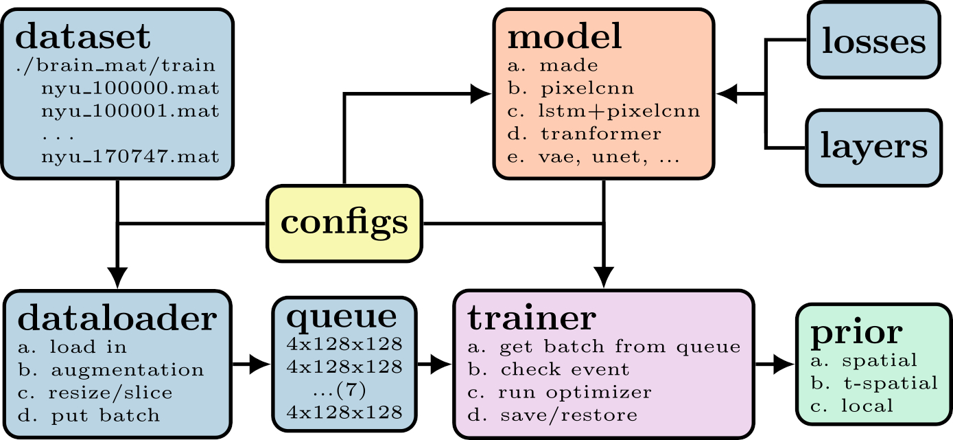
We trained the neural network $$$\mathrm{NET}(\hat{\Theta}, \boldsymbol{x})$$$ with TensorFlow, exported the computation graph, and saved the trained model. The workflow to train a prior is illustrated in Figure 1. The input node and the loss node of a computation graph, corresponding to the image $$$\boldsymbol{x}$$$ and the log-likelihood regularization term $$$R_{logp}(\boldsymbol{x})$$$, respectively, were wrapped in BART's non-linear operator (nlop). The forward pass and the gradient of $$$R_{logp}(\boldsymbol{x})$$$ are called via nlop's forward function and adjoint function, respectively.The initialization of an exported TensorFlow graph, the restoration of a saved model, and the inference are implemented with TensorFlow's C API whose libraries were downloaded from TensorFlow's official page [6]. The dependencies on CUDA and cuDNN for TensorFlow are satisfied with Conda [7]. The system matrix $$$\mathcal{A}$$$ already existed in BART. FISTA [8] was used to solve Eq (1). The proximal operation on $$$R_{logp}(\boldsymbol{x})$$$ was approximated with gradient update. The learned log-likelihood prior was presented to the user as a regularization option for the reconstruction command. The usage is as follow:
$$\texttt{bart pics -R LP:\{model_path\}:$\lambda$:pct:n <kspace> <sensitivities> <output>}, $$where $$$\texttt{pct}$$$ is the update percentage and the $$$\texttt{n}$$$ specifies how many times the gradient inference runs for every FISTA iteration.
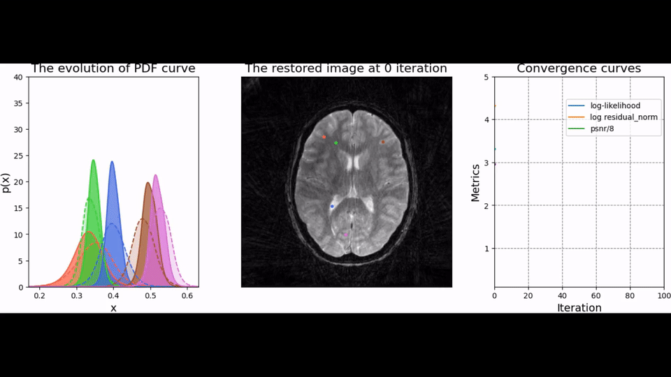
To test the trained prior, we reconstructed the image from simulated radial k-space data and tracked peak signal-to-noise ratio, residual norm, and bits/pixel over iterations following the approach proposed in [5] (cf, Figure 2). At last, the developed pipeline was used to reconstruct an image of a human brain from prospectively sampled radial k-space data (Figure 3).
Results
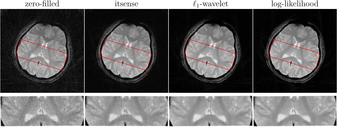
The developed pipeline was used to reconstruct images from prospectively sampled radial k-space data. As shown in Figure 3, the reconstruction regularized by the learned log-likelihood model has the best noise suppression and the clearest boundaries between different tissues.Conlusions
The BART toolbox is a flexible framework for the integration of the trained neural network model. Based on existing functionality, the deep image prior can be conveniently added to different reconstruction pipelines.Acknowledgements
Supported by the DZHK (German Centre for Cardiovascular Research). We gratefully acknowledge funding by the "Niedersächsisches Vorab" initiative of the Volkswagen Foundation and funding by NIH under grant U24EB029240. We acknowledge the support of the NVIDIA Corporation with the donation of one NVIDIA TITAN Xp GPU for this research. At last, the sincere gratitude to colleagues for insightful discussions and suggestions.References
[1] Uecker M et al., BART Toolbox for Computational Magnetic Resonance Imaging, DOI:10.5281/zenodo.592960
[2] Abadi M et al., TensorFlow: Large-Scale Machine Learning on Heterogeneous Systems
[3] Block KT et al. ”Undersampled radial MRI with multiple coils. Iterative image reconstruction using a total variation constraint.” Magnetic Resonance in Medicine: An Official Journal of the International Society for Magnetic Resonance in Medicine 57.6 (2007):1086-1098.
[4] Michael L et al. ”Compressed sensing MRI.” IEEE signal processing magazine 25.2(2008): 72-82.
[5] Luo G et al., ”MRI reconstruction using deep Bayesian estimation.” Magnetic Resonance in Medicine 84.4 (2020): 2246-2261.
[6] https://www.TensorFlow.org/install/lang_c
[7] Anaconda Software Distribution. (2020). Anaconda Documentation. Anaconda Inc. Retrieved from https://docs.anaconda.com/
[8] Beck A and Teboulle M. ”A fast iterative shrinkage-thresholding algorithm for linear inverse problems.” SIAM journal on imaging sciences 2.1 (2009): 183-202.
[9] Rosenzweig S, Holme HCM, Uecker M. ”Simple auto‐calibrated gradient delay estimation from few spokes using Radial Intersections (RING).” Magnetic resonance in medicine 81.3 (2019): 1898-1906.
[10] Salimans, Tim, et al. "Pixelcnn++: Improving the pixelcnn with discretized logistic mixture likelihood and other modifications." arXiv preprint arXiv:1701.05517 (2017).
Figures