0794
The Effect of Oblique Image Slices on the Accuracy of Quantitative Susceptibility Mapping and a Robust Tilt Correction Method1Department of Medical Physics and Biomedical Engineering, University College London, London, United Kingdom, 2UCL Queens Square Institute of Neurology, London, United Kingdom
Synopsis
Quantitative susceptibility mapping (QSM) using the MRI phase to calculate tissue magnetic susceptibility is finding increasing clinical applications. Oblique image slices are often acquired to facilitate radiological viewing and reduce artifacts. Here, we show that artifacts and errors arise in susceptibility maps if oblique acquisition is not properly taken into account in QSM. We performed a comprehensive analysis of the effects of oblique acquisition on brain susceptibility maps and compared tilt correction schemes for three susceptibility calculation methods, using a numerical phantom and human in-vivo images. We demonstrate a robust tilt correction method for accurate QSM with oblique acquisition.
Introduction
Quantitative susceptibility mapping (QSM) is finding increasing clinical applications. Acquisition of oblique image slices is common clinical practice to facilitate radiological viewing but pilot studies suggest this gives incorrect susceptibility ($$$\chi$$$) estimates when unaccounted for1. Using a numerical brain phantom2, we performed a comprehensive analysis of the effects of oblique acquisition and compared proposed tilt correction methods for the final $$$\chi$$$ calculation step in the QSM pipeline. We confirmed these results in vivo, and demonstrate a robust tilt correction method for accurate $$$\chi$$$ calculation.Methods
Numerical Phantom:Local field maps were obtained from a non-linear fit3 over echo times of complex data, created from magnitude and phase images of a numerical brain phantom2, with no background fields. These background-field-free maps were used to independently analyse the $$$\chi$$$ calculation step in the QSM pipeline without confounds from phase unwrapping or background field removal. To simulate oblique slice acquisition, the untilted reference local field map (at 0°) was tilted by -45° to +45° in 5° steps. All rotations were carried out about the x-axis (u-axis, Figure 1) using FSL FLIRT4 with trilinear interpolation.
We tested four proposed tilt correction schemes (Figure 1):
- RotPrior: image rotated into scanner frame prior to $$$\chi$$$ calculation (with a k-space dipole defined in the scanner frame)
- DipK: image left unaligned (k-space dipole defined in the tilted image frame)
- DipIm: image left unaligned (image-space dipole defined in the tilted image frame)
- NoRot: image left unaligned (simulating mistaken definition of the k-space dipole in the scanner frame misaligned to the tilted image)
In Vivo:
3D gradient-echo brain images of a healthy volunteer were acquired on a 3T Siemens Prisma MR system (National Hospital for Neurology and Neurosurgery, London, UK) using a 64-channel head coil. The image volume was tilted about the x-axis from -20° to +20° in 5° increments and acquired in 3 min 23 s (per volume) with TE1/ΔTE/TE5 = 4.92/4.92/24.60ms; TR=30ms; 1.23 mm isotropic voxels; 6/8 partial Fourier; and GRAPPAPE acceleration = 3.
For all angles/volumes, a total field map and noise map were obtained using a non-linear fit of the complex data3. A brain mask was created using BET12,13, eroded by 6 voxels, and multiplied with a mask created by thresholding the inverse noise map at its mean to remove noisy voxels. Residual phase wraps were removed using Laplacian unwrapping13,14 and background fields were removed using the Laplacian boundary value (LBV)13,15 technique as it is independent of tilt angle. The four tilt correction schemes were compared using the same three $$$\chi$$$ calculation methods as for the numerical phantom.
For each angle, the magnitude image (RMS across echoes) was rigidly registered to the reference (0°) using NiftyReg16 and the transformation matrix was used to transform the $$$\chi$$$ maps into the reference space for comparison. ROIs were obtained by registering the EVE17 magnitude image with the same reference image and applying the resulting transformation to the EVE ROIs. Mean $$$\chi$$$ values were calculated in these ROIs for all angles. RMSE and XSIM were also used to compare tilt-corrected maps with the 0° reference susceptibility map.
Results
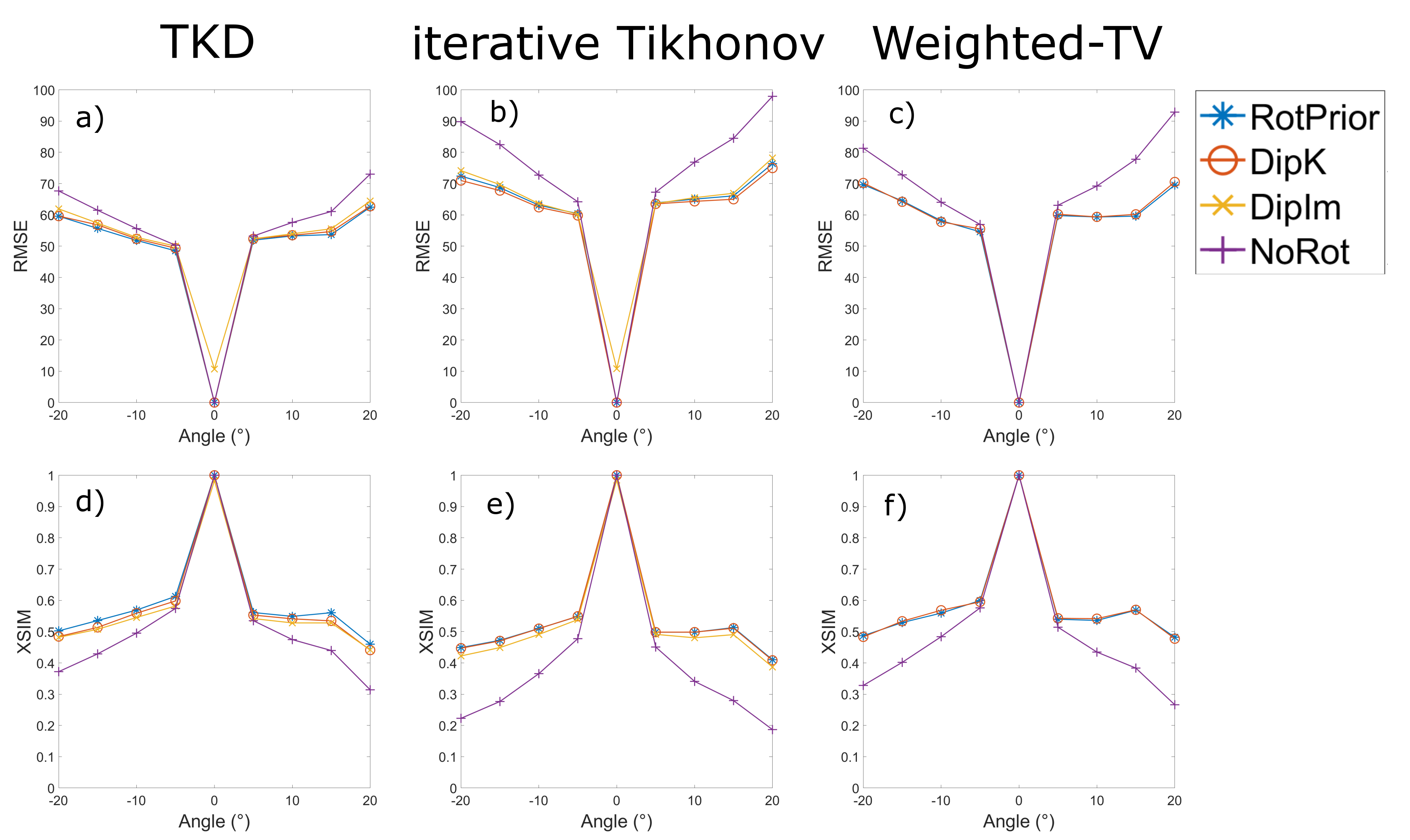
Numerical Phantom:All QSM methods are most accurate with RotPrior, and least accurate with NoRot when the dipole is misaligned to the main magnetic field (Figure 2). wlTV is relatively robust to oblique acquisition, with RotPrior and DipK performing similarly. However, DipK shows variability in $$$\chi$$$ across angles in different ROIs. $$$\chi$$$ maps (Figure 3) make clearly apparent the errors resulting from NoRot.
In Vivo:
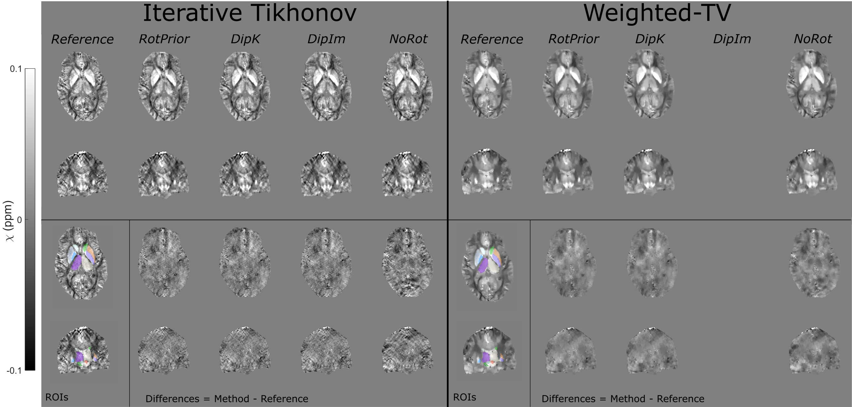
Figure 4 confirms that NoRot results in large susceptibility errors and that RotPrior is comparable to DipK between $$$\pm$$$20°, both performing better than DipIm, in agreement with the phantom results. Difference images also confirm the phantom results (Figure 5). Subtle effects found in the phantom ROIs (Figure 2) were not apparent in vivo (not shown) due to noise, motion, rotation/registration interpolation effects and the expected variability in QSMs over repeated acquisitions18.
Conclusions
We have shown that, for any susceptibility calculation method (TKD, iterative Tikhonov and wlTV) applied to an oblique acquisition, leaving the dipole kernel misaligned with the main magnetic field ($$$\mathbf{\hat{B}}_0$$$) direction, which is often the default mode of QSM toolboxes, leads to substantial $$$\chi$$$ errors. The most accurate susceptibilities can be obtained when local field maps are rotated into alignment with the scanner axes prior to $$$\chi$$$ calculation (RotPrior). For wlTV, accurate susceptibility calculation can be carried out in the tilted image frame without any rotations provided the correct ($$$\mathbf{\hat{B}}_0$$$) direction is used in defining the k-space dipole (DipK).Acknowledgements
Oliver Kiersnowski is supported by the EPSRC-funded UCL Centre for Doctoral Training in Intelligent, Integrated Imaging in Healthcare (i4health) (EP/S021930/1). Karin Shmueli is supported by ERC Consolidator Grant DiSCo MRI SFN 770939. We thank Dr Carlos Milovic for his assistance with FANSI.References
- Dixon EC. Applications of MRI Magnetic Susceptibility Mapping in PET-MRI Brain Studies. Dr thesis, UCL (University Coll London). 2018. http://discovery.ucl.ac.uk/10053515/.
- Marques, José P., et al. "QSM Reconstruction Challenge 2.0 Part 1: A Realistic in silico Head Phantom for MRI data simulation and evaluation of susceptibility mapping procedures." bioRxiv (2020).
- Liu T, Wisnieff C, Lou M, Chen W, Spincemaille P, Wang Y. Nonlinear formulation of the magnetic field to source relationship for robust quantitative susceptibility mapping. Magn Reson Med. 2013 Feb;69(2):467-76. doi: 10.1002/mrm.24272. Epub 2012 Apr 9. PMID: 22488774.
- Jenkinson M, Beckmann CF, Behrens TEJ, Woolrich MW, Smith SM. FSL. Neuroimage. 2012;62:782-790. doi:10.1016/j.neuroimage.2011.09.015
- Shmueli K, De Zwart JA, Van Gelderen P, Li TQ, Dodd SJ, Duyn JH. Magnetic susceptibility mapping of brain tissue in vivo using MRI phase data. Magn Reson Med. 2009;62(6):1510-1522. doi:10.1002/mrm.22135
- Karsa, A, Punwani, S, Shmueli, K, et al. An optimized and highly repeatable MRI acquisition and processing pipeline for quantitative susceptibility mapping in the head‐and‐neck region. Magn Reson Med. 2020; 84: 3206– 3222. https://doi.org/10.1002/mrm.28377
- PMID: 32621302.MRI susceptibility calculation methods. https://xip.uclb.com/i/software/mri_qsm_tkd.html.
- Schweser F, Deistung A, Sommer K, Reichenbach JR. Toward online reconstruction of quantitative susceptibility maps: Superfast dipole inversion. Magn Reson Med. 2013;69(6):1581-1593. doi:10.1002/mrm.24405
- Bilgic B., Chatnuntawech I., Langkammer C., Setsompop K.; Sparse Methods for Quantitative Susceptibility Mapping; Wavelets and Sparsity XVI, SPIE 2015
- Milovic C, Bilgic B, Zhao B, Acosta-Cabronero J, Tejos C. Fast Nonlinear Susceptibility Inversion with Variational Regularization. Magn Reson Med. Accepted Dec. 12th 2017. DOI: 10.1002/mrm.27073
- Milovic C, Tejos C, and Irarrazaval P. Structural Similarity Index Metric setup for QSM applications (XSIM). 5th International Workshop on MRI Phase Contrast & Quantitative Susceptibility Mapping, Seoul, Korea, 2019.
- S.M. Smith. Fast robust automated brain extraction. Human Brain Mapping, 17(3):143-155, November 2002.
- http://pre.weill.cornell.edu/mri/pages/qsm.html
- Schofield, Marvin A., and Yimei Zhu, ‘Fast Phase Unwrapping Algorithm for Interferometric Applications’, Optics Letters, 2003 https://doi.org/10.1364/ol.28.001194
- Zhou, Dong, Tian Liu, Pascal Spincemaille, and Yi Wang, ‘Background Field Removal by Solving the Laplacian Boundary Value Problem’, NMR in Biomedicine, 27.3 (2014), 312–19 <https://doi.org/10.1002/nbm.3064>
- Modat, et al. (2014). Global image registration using a symmetric block-matching approach. Journal of Medical Imaging, 1(2), 024003–024003. doi:10.1117/1.JMI.1.2.024003
- Lim IA, Faria AV, Li X, Hsu JT, Airan RD, Mori S, van Zijl PC. Human brain atlas for automated region of interest selection in quantitative susceptibility mapping: application to determine iron content in deep gray matter structures. Neuroimage. 2013 Nov 15;82:449-69. doi: 10.1016/j.neuroimage.2013.05.127. Epub 2013 Jun 12. PMID: 23769915; PMCID: PMC3966481.
- Xiang Feng, Andreas Deistung, Jürgen R. Reichenbach,Quantitative susceptibility mapping (QSM) and R2* in the human brain at 3T: Evaluation of intra-scanner repeatability, Zeitschrift für Medizinische Physik, Volume 28, Issue 1, 2018, Pages 36-48
Figures
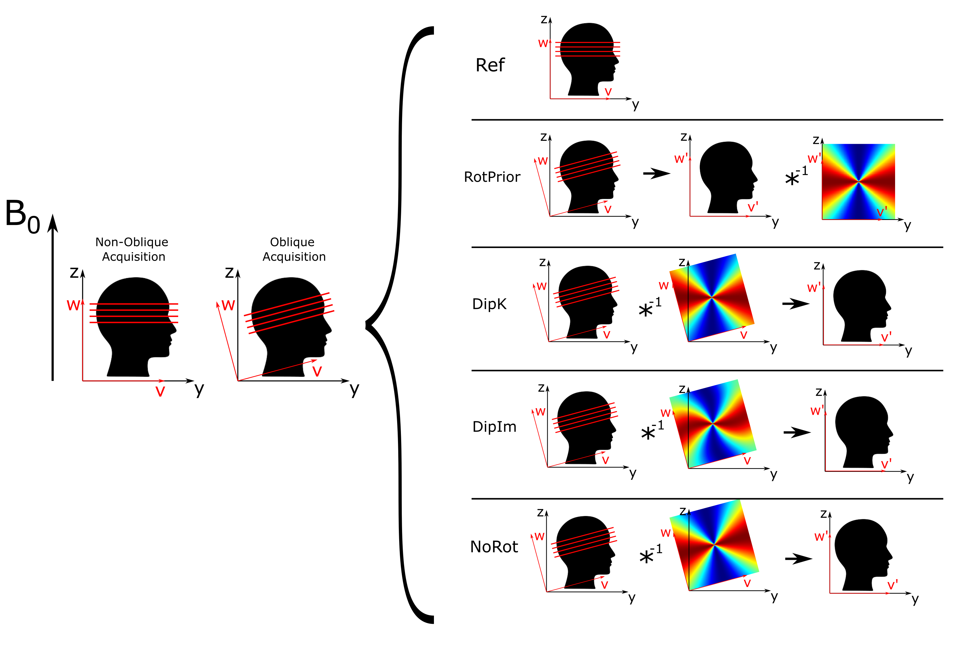
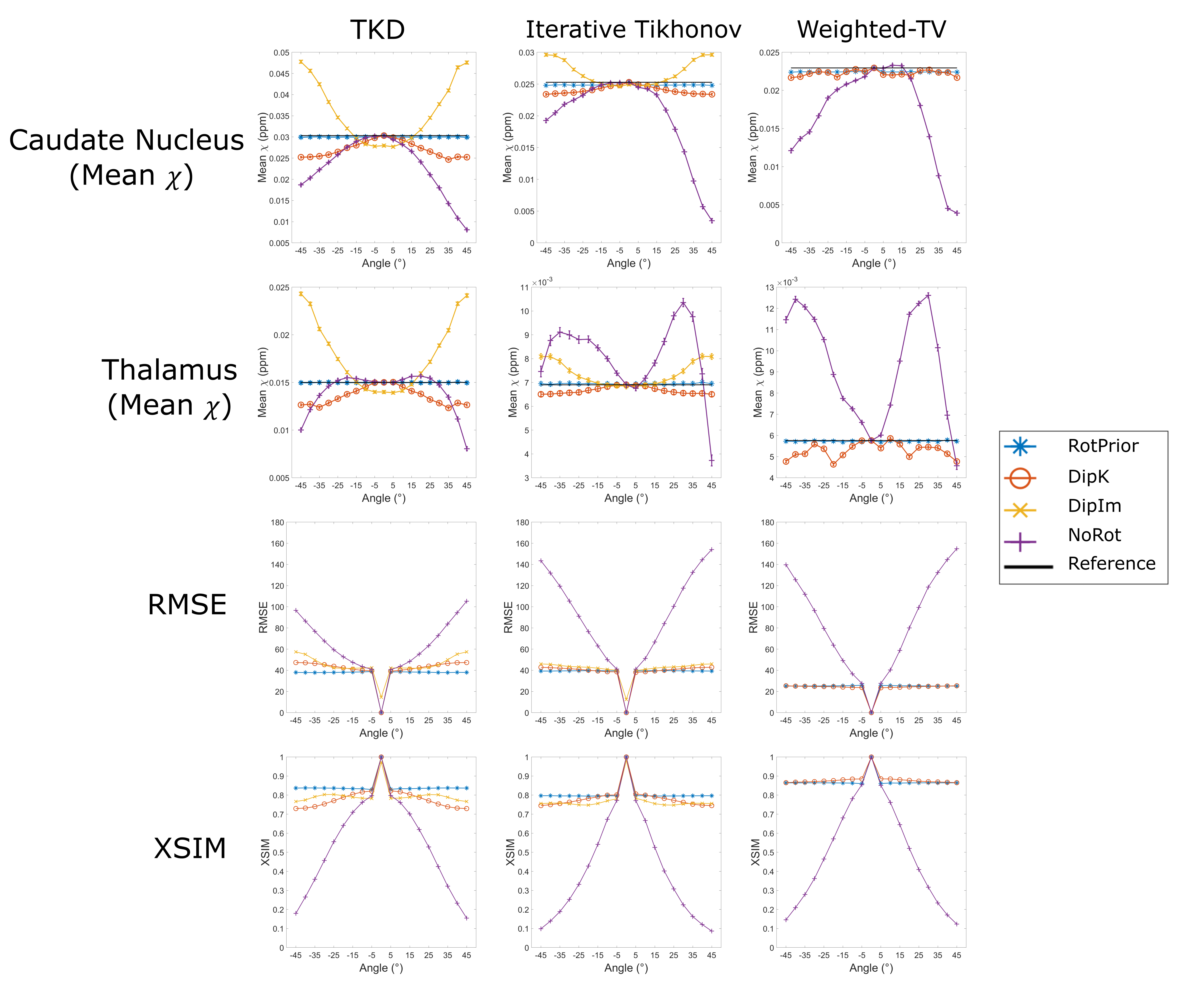
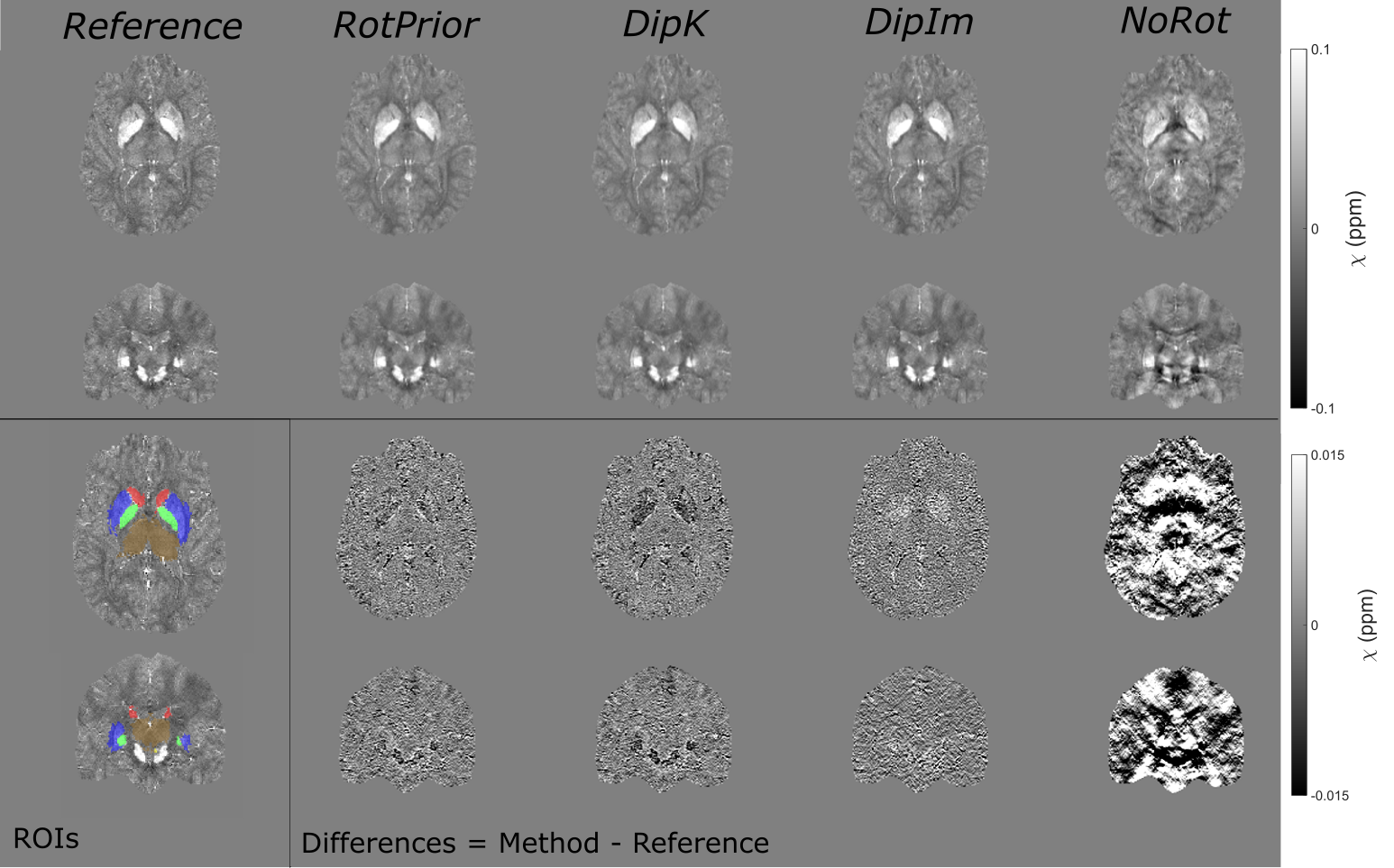
Figure 3: $$$\chi$$$ maps and difference images illustrating the effects of all tilt correction schemes in the numerical phantom. An axial and a coronal slice are shown for a volume tilted at 25° and a reference 0° volume with all $$$\chi$$$ maps calculated using the iterative Tikhonov method. The ROIs analysed are also shown (bottom left). Qualitatively, RotPrior performs the best while NoRot results in substantial $$$\chi$$$ errors across the whole brain. The results from TKD and weighted linear TV (not shown) are very similar.