0497
A computational fluid dynamics framework to generate digital reference objects for perfusion imaging
Ulin Nuha Abdul Qohar1, Erik Andreas Hanson1, Steven Sourbron2, and Antonella Zanna Munthe-Kaas1
1Mathematics, University of Bergen, Bergen, Norway, 2University of Sheffield, Sheffield, United Kingdom
1Mathematics, University of Bergen, Bergen, Norway, 2University of Sheffield, Sheffield, United Kingdom
Synopsis
In this study, we present a simulation framework capable of generating synthetic reference perfusion MRI data suitable for evaluation and comparison of tracer kinetic models. The framework consists of a graph-based contrast agent flow model with a vascular geometry and allows for controlled simulations with realistic structural and vascular parameters. We demonstrate the potential application of the proposed framework by performing a comparison between traditional pharmacokinetic models of varying complexity, by studying the effect of ROI size.
INTRODUCTION
Perfusion estimates from dynamic contrast-enhanced magnetic resonance imaging (DCE-MRI) or arterial spin labelling (ASL) have been proposed for diagnosis, prognosis and monitoring of disease progression and intervention.1-5 Such perfusion estimations rely on black-box tracer-kinetic models6-8 and may be vulnerable to systematic errors4 depending on the model assumptions and parameter choices. In this work, we present a computational fluid dynamics (CFD) framework for generating synthetic perfusion imaging data. The proposed model can act as a digital reference object with controlled ground-truth parameters. It can be used to study the effect of model assumptions and other processing steps such as, for instance, the effect of ROI placement.METHODS
CFD model:The proposed model is based on a coupling between components on various spatial scales. The observable vascular networks above 30-micron radius were described using graph model9 and the microvasculature was represented by a fractal network model. Both components were based on Poisseuille's law representing the vessel resistance. In addition, we assumed no leakage from the system. The pressure differences related to node $$$i$$$ can be written as
$$ \sum_{j \in N_i} R_{ij}\gamma \left(P_i-P_j\right) = q_i,$$
where $$$N_i, R_{ij}, \gamma$$$, and $$$q_i$$$ are the connected neighbour nodes to node $$$i$$$, the vessel resistance, the capillary resistance constant(1 for arteries and veins) and the inlet/outlet flow to the node $$$i$$$ (zero for inner nodes), respectively.
Contrast agent (CA) flow:
The contrast agent was assumed to move passively with the bloodstream obtained from the graph model. The CA influx into a small distribution volume $$$\Omega_k$$$ was defined by the product of CA concentration ($$$C_k$$$) and blood flow influx ($$$\textbf{q}_k$$$). It is equivalent to the CA change rate in the distribution volume $$$\Omega_k$$$
$$\frac{d}{dt}\int_{\partial \Omega_k}Cd\textbf{x} = -\frac{1}{\Omega_k} \int_{\partial \Omega_k}C_k (\textbf{q}_k \cdot \textbf{n}) d\textbf{x},$$
where index $$$k$$$ represents a segment in arteries, veins and capillaries. A bolus injection in the arterial root vessel was simulated using a gamma variate function,
$$C_{AIF}(t)=C_0(t - t_0)A.e^{-(t-t_0)/B}$$
for constants $$$t_0 = 6$$$s; $$$A = 3; B = 1; C_0 = 1$$$mM.10
Numerical experiments:
For illustration, the approach was used to build a CFD model based on a frog tongue vasculature segmentation (Figure 1). The blood circulation was obtained by solving the model based on equation (1). A synthetic perfusion series with a total acquisition time of 120s was generated using the steps outlined above.
The images were analyzed using four models: Maximum Slope (MS), One-compartment Model (1CM), two-compartment Uptake (2CUM) and Exchange Model (2CXM)5-7 These models are commonly used for quantification of plasma flow (PF) and plasma volume (PV). Reconstructed values for these parameters were compared to the blood flow extracted from the ground truth data. Three different questions were addressed to illustrate the power of the approach: a comparison of analyses with local and global AIFs, a comparison of kinetic models, and an evaluation of the effect of ROI selection. Figure 1 shows the 11 ROIs used for this study.
RESULTS
Figure 2 shows that the CA propagation has the expected behaviour as it flows from the arterial network roots feeding the whole vasculature, spreads to the capillaries and is washed out through the veins. Figure 3 shows the CA signal, which reveals a short CA delay after bolus injection. In addition, four model fits: the MS fit describes the up-slope well; the other three model fits are almost identical.Figure 4 shows the error in the PF values for each model with a local AIF. The MS model was systematically underestimating PF values. Both the 2C models and the 1C gave similar results for all ROIs, except in ROI 2. This is not unexpected since the model considers intravascular CA only and the kinetics is therefore essentially one-compartmental in nature. Figure 5 shows that the global AIF yields lower PF estimation, consistent with the effects of bolus dispersion.
PV estimation results from 2CXM and 2CUM with local AIFs were relatively accurate with the average error of 4% and 3.9%, respectively. The estimations were robust to AIF selection with the global AIF giving a slightly larger average error (4.7% and 4.4%).
DISCUSSION
We proposed a CFD-based framework to generate computational models of macrovascular and microvascular blood flow and tracer kinetics in a realistic vascular network. We hypothesized that this may provide synthetic ground truth data to compare different perfusion MRI modelling and analysis approaches. We explored the potential of this approach by application to a simple 2D example and by investigating well-known problems of kinetic model selection, AIF selection and ROI selection. We demonstrated that this produces data with the expected behaviour and results that are qualitatively in line with the current understanding of these issues. But unlike previous studies into model dependence, the setup does not rely on synthetic ground truth data that themselves are modelled using simplified black box models.CONCLUSION
Preliminary experiments show that the proposed CFD framework provides suitable ground truth data that can be used to study the elusive problem of model bias in more depth than was previously possible. Future research will require more in-depth studies with fine-grained vascular networks and a more accurate simulation of key imaging features such as limited spatial resolution and partial volume effects.Acknowledgements
No acknowledgement found.References
- Kallehauge, J. F., Tanderup, K., Duan, C., et al. Tracer kinetic model selection for dynamic contrast-enhanced magnetic resonance imaging of locally advanced cervical cancer. Acta Oncologica, 2014; 53(8): 1064-1072.
- Gaa, T., Neumann, W., Sudarski, S., et al. Comparison of perfusion models for quantitative T1 weighted DCE-MRI of rectal cancer. Scientific Reports, 2017; 7(1): 1-9.
- Rasti, R., Teshnehlab, M., & Phung, S. L. Breast cancer diagnosis in DCE-MRI using mixture ensemble of convolutional neural networks. Pattern Recognition, 2017;72: 381-390.
- Peled, S., Vangel, M., Kikinis, R., et al. Selection of fitting model and arterial input function for repeatability in dynamic contrast-enhanced prostate MRI. Academic radiology, 2019;26(9): e241-e251.
- Ingrisch, M., & Sourbron, S. Tracer-kinetic modelling of dynamic contrast-enhanced MRI and CT: a primer. Journal of pharmacokinetics and pharmacodynamics, 2013; 40(3): 281-300.
- Sourbron, S. P. and Buckley, D. L. Classic models for dynamic contrast‐enhanced MRI. NMR in Biomedicine, 2013;26(8): 1004-1027.
- Koh, T. S., Bisdas, S., Koh, D. M., & Thng, C. H. Fundamentals of tracer kinetics for dynamic contrast‐enhanced MRI. Journal of Magnetic Resonance Imaging, 2011;34(6): 1262-1276.
- Khalifa, F., Soliman, A., El‐Baz, A., et al. Models and methods for analyzing DCE‐MRI: A review. Medical physics, 2014;41(12): 124301.
- Reichold, J., Stampanoni, M., Keller, A. L., et al. Vascular graph model to simulate the cerebral blood flow in realistic vascular networks. Journal of Cerebral Blood Flow & Metabolism, 2009;29(8): 1429-1443.
- Hodneland, E., Hanson, E., Sævareid, O., et al. A new framework for assessing subject-specific whole-brain circulation and perfusion using MRI-based measurements and a multi-scale continuous flow model. PLoS computational biology, 2019;15(6): e1007073.
Figures
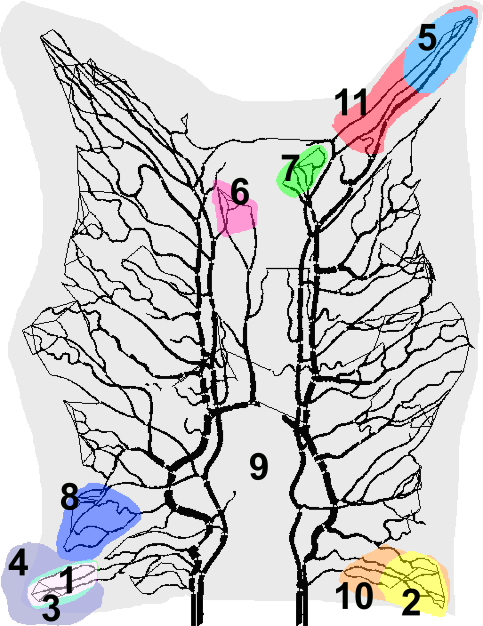
The segmented vascular structures and ROIs in the experiment: Each colour represents a different ROI. Several ROIs are overlapping (ROI 1,3, and 4; 2 and 10; and 5 and 11) for error analysis in similar areas with different ROI size. ROI 6 and 7 are the two regions with biggest error among 11 ROIs, and the blue region (ROI 8) has the most accurate estimation for both one and two-compartments model.
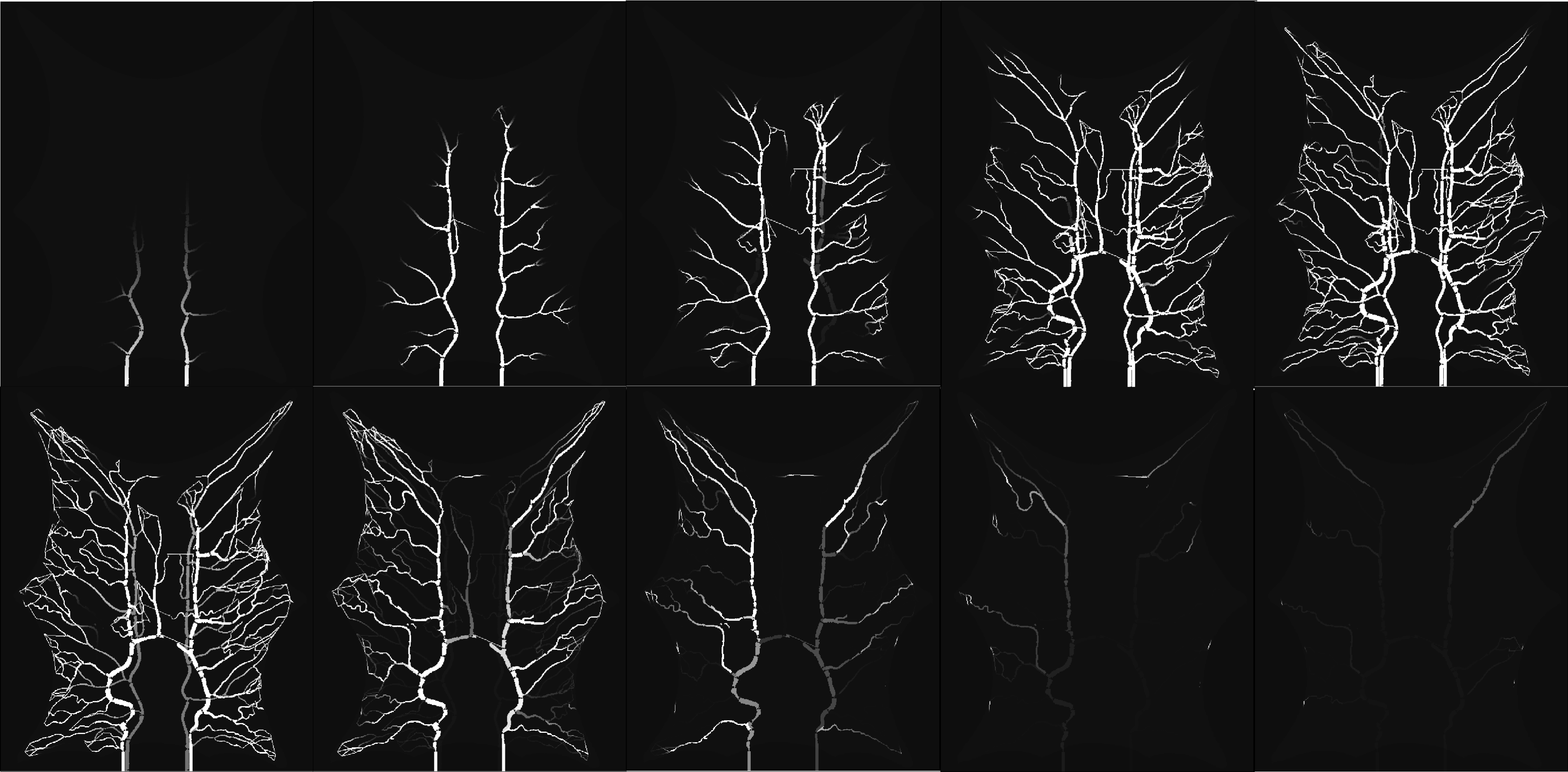
Simulated CA flow in the vascular system after bolus injection. The flow patterns exhibit a natural behaviour with a flow from the arterial network roots feeding the whole vasculature, spreading to the capillaries and a washout through the veins. The images were captured at 6, 8, 10, 15, 20, 25, 35, 50, 70 and 100 second respectively (from left to right).
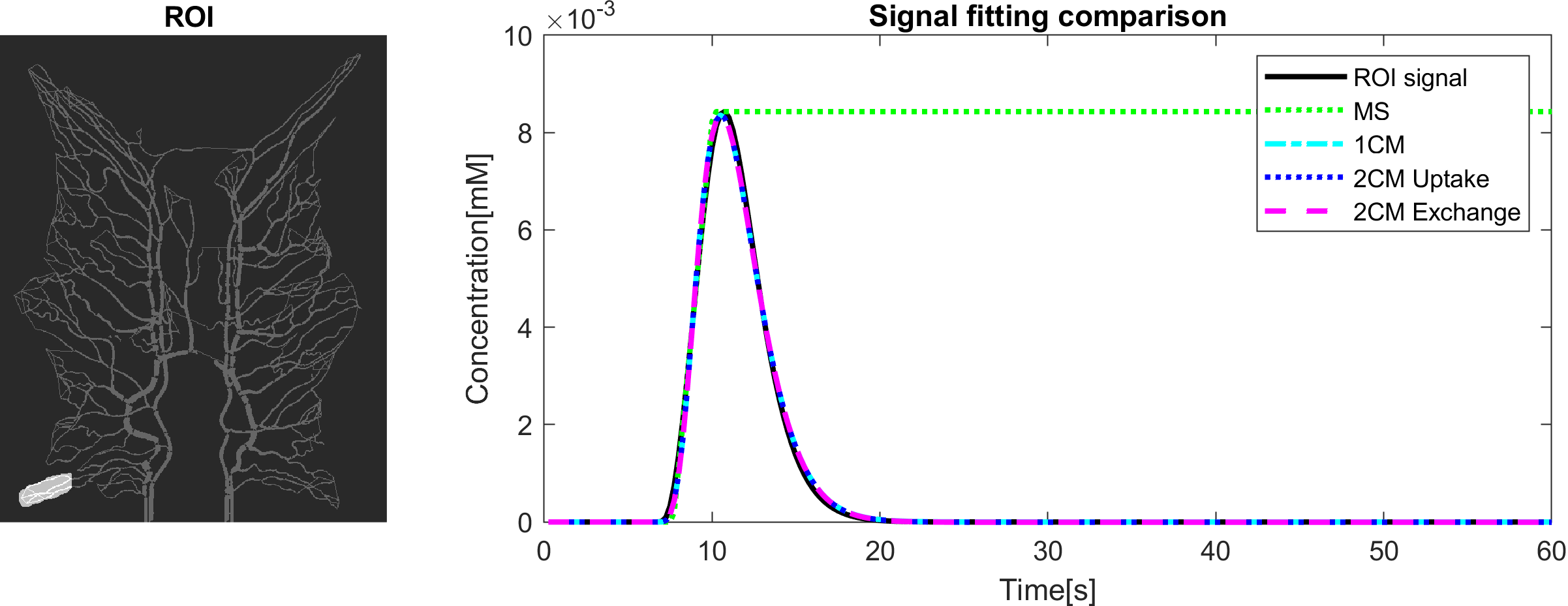
The simulated CA signal without noise averaged over ROI 1. The curve indicates the CA concentration from 0s to 60s acquisition time, which shows a short CA delay after bolus injection. This data is resembling the perfusion signal in clinical imaging. Four tracer kinetic models were used for quantifying perfusion from the time curve using a local AIF. The signal fittings for all models were well-performed with good fitting. MS fitting reveals the CA curve's maximum slope location and the slope magnitude and the remaining fittings coincide and generate an identical result.
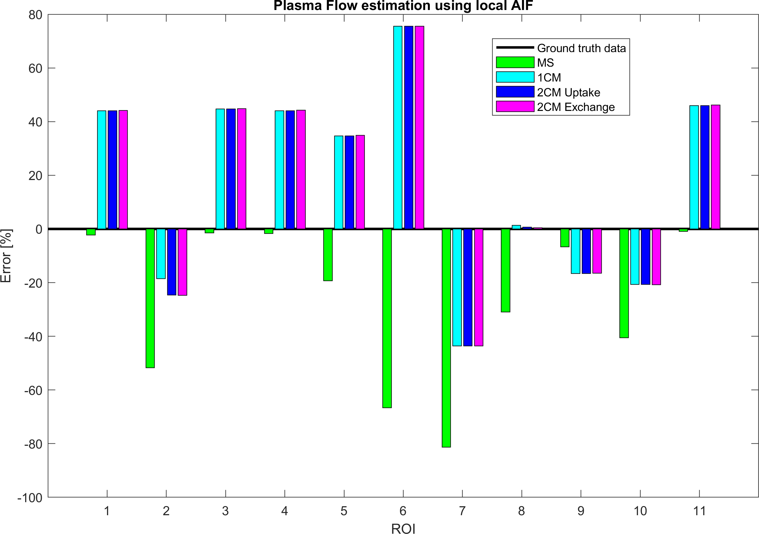
Plasma flow (PF) estimation results using four tracer kinetic models in 11 ROIs. The MS model is systematically underestimating PF, but generate the best estimation among the four models in terms of absolute values. The remaining models are, in general, overestimating PF and generate close to identical values, except for ROI 2. This reveals that the 2-compartment models are over-parameterized and not suited for estimations in our CA flow phantom. The proposed flow model only accounts for blood circulation in the intravascular structures.
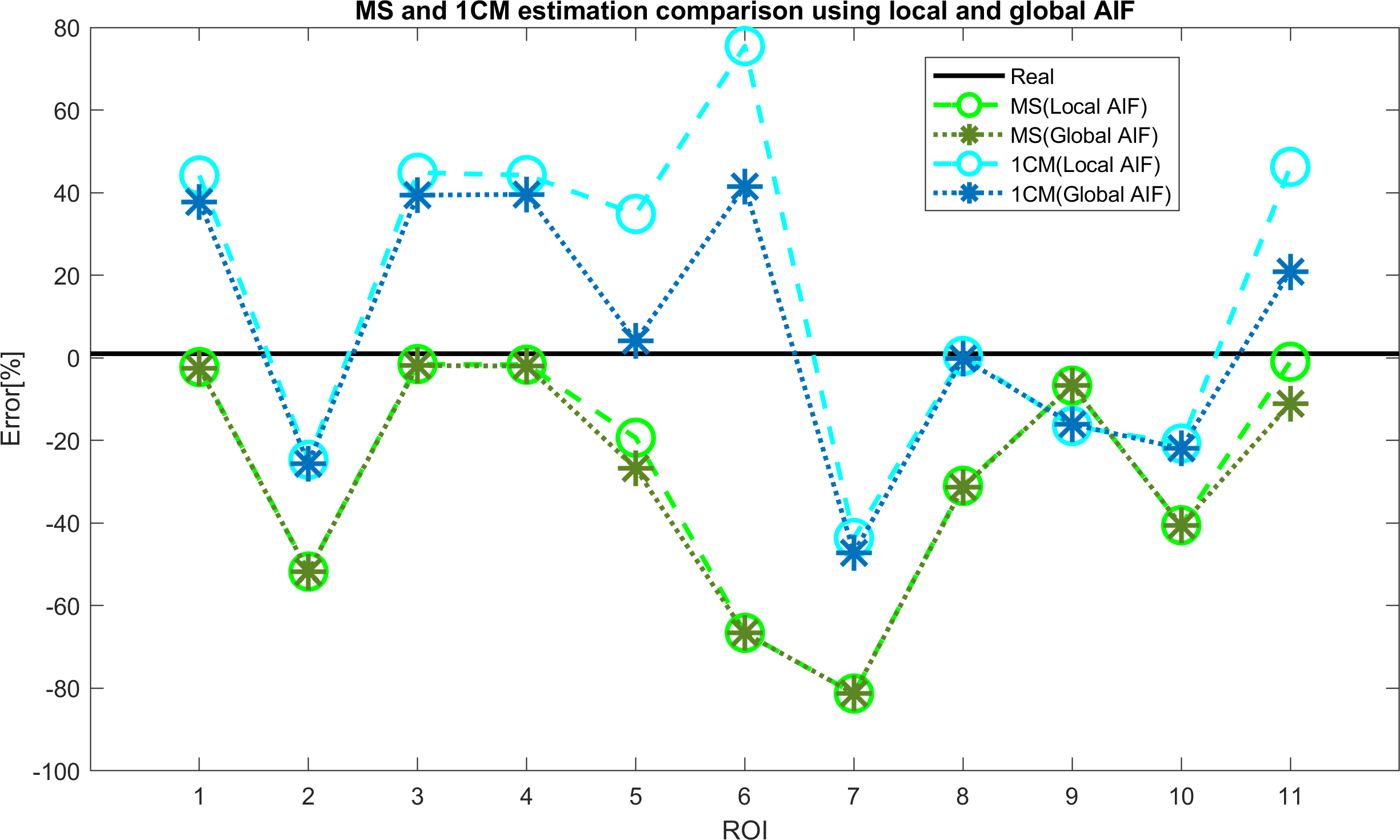
Since both 2CXM and 2CUM estimation results were almost identic with the 1CM. Only 1CM and MS fitting were analyzed for comparison between local and global AIF. PF estimation using a global AIF is in general lower than for a local AIF. It provides smaller errors for 1CM (due to overestimating) and larger errors for MS conversely. These results may be caused by bolus dispersion and are related to the distance between the location of global and local AIF. The global AIF has a higher concentration peak and longer delay to the ROI, compared to local AIF.