0271
Can Un-trained Networks Compete with Trained Ones for Accelerated MRI?1Electrical and Computer Engineering, Rice University, Houston, TX, United States, 2Electrical and Computer Engineering, Technical University of Munich, Munich, Germany
Synopsis
Convolutional Neural Networks (CNNs) are highly effective tools for image reconstruction problems. Typically, CNNs are trained on large amounts of images, but, perhaps surprisingly, even without any training data, CNNs such as the Deep Image Prior and Deep Decoder achieve excellent imaging performance. Here, we build on those works by proposing an un-trained CNN for accelerated MRI along with performance-enhancing steps including enforcing data-consistency and combining multiple reconstructions. We show that the resulting method i) achieves reconstruction performance almost on par with baseline as well as state-of-the-art trained CNNs, but without any training, and ii) significantly outperforms competing sparsity-based approaches.
Introduction
Convolutional Neural Networks (CNN) including Variational Networks1 and even a simple U-net2 trained on a large set of training images outperform classical sparsity-based methods for accelerated Magnetic Resonance Imaging (MRI). Almost exclusively, CNNs are trained on large sets of images. However, this dependence on training data can be problematic because (i) CNNs often suffer a performance loss when being applied to out-of-distribution examples, and (ii) it is difficult to apply them in clinical applications where only little training data is available.In this work, we study accelerating multi-coil MRI with un-trained CNNs that do not rely on any training data. In very recent work, it has been demonstrated that un-trained CNNs such as the Deep Image Prior3 (DIP) and Deep Decoder4 (DD) enable reconstruction of images from few and noisy measurements5,6. However, those previous works obtained images that are too smooth and contain artifacts, which results in worse performance compared to trained CNNs. In this work, we aim to overcome those issues towards closing the performance gap to trained networks.
Methods
The ConvDecoder, depicted in Figure 1, is a generative convolutional neural network that maps a parameter space to images, i.e., $$$G: \mathbb{R}^p \to \mathbb{R}^{c \times w \times h}$$$, where $$$c$$$ is the number of output channels, and $$$w$$$ and $$$h$$$ are the width and height of the image in each channel. The input of the network is chosen randomly, is fixed, and functions as a seed. The parameters of the network are the weights of the convolutional layers.We are given the k-space measurements $$$\mathbf{y}_1,\ldots,\mathbf{y}_{n_c}$$$ of $$$n_c$$$ receiver coils undersampled with a given mask $$$\mathbf{M}$$$ of an unknown image, and our goal is to estimate the image. We reconstruct an image as follows:
Step 1: Apply the first-order gradient method Adam7 starting from a random initialization $$$\mathbf{C}_0$$$ to minimizing the loss function
$$
\mathcal{L}(\mathbf{C}) = \frac{1}{2} \sum_{i=1}^{n_c} \lVert \mathbf{y}_i - \mathbf{M} \mathbf{F} G_i(\mathbf{C}) \rVert_2^2.
$$
Here, $$$\mathbf{F}$$$ is the 2D Fourier transform, and $$$G_i$$$ is the $$$i$$$-th output channel of the ConvDecoder.
Step 2: Enforce data consistency of the resulting images $$$G_i(\mathbf{C})$$$.
Step 3: Combine the images $$$G_i(\mathbf{C})$$$ via the root-least-squares algorithm to a single image.
Step 4: Repeat Steps 1-3 k-times, with different random initializations of the ConvDecoder and average the results.
The new elements of this approach relative to previous works are i) the ConvDecoder architecture ii) the data-consistency step, and iii) the ensembling trick (step 4). The ConvDecoder is a variation of the Deep Decoder architecture and results in slightly less blurry reconstructions and the data-consistency and ensembling steps each improves performance notably for all architectures we considered.
Note that this method works without any estimates of the sensitivity maps. We also considered a slight variation of the method which takes the sensitivity maps estimated with ESPIRIT8 into account in the loss function above. We found the method above to work best for knee images, and the variant with sensitivity map estimates to work best for brain images.
We study the performance of this method on the Knee and Brain FastMRI dataset. We compared to Total-Variation norm minimization9 (TV) as a conventional sparsity-based method, to U-net as a baseline trained network, and to VarNet because it is the best-performing method on the FastMRI dataset.
Results
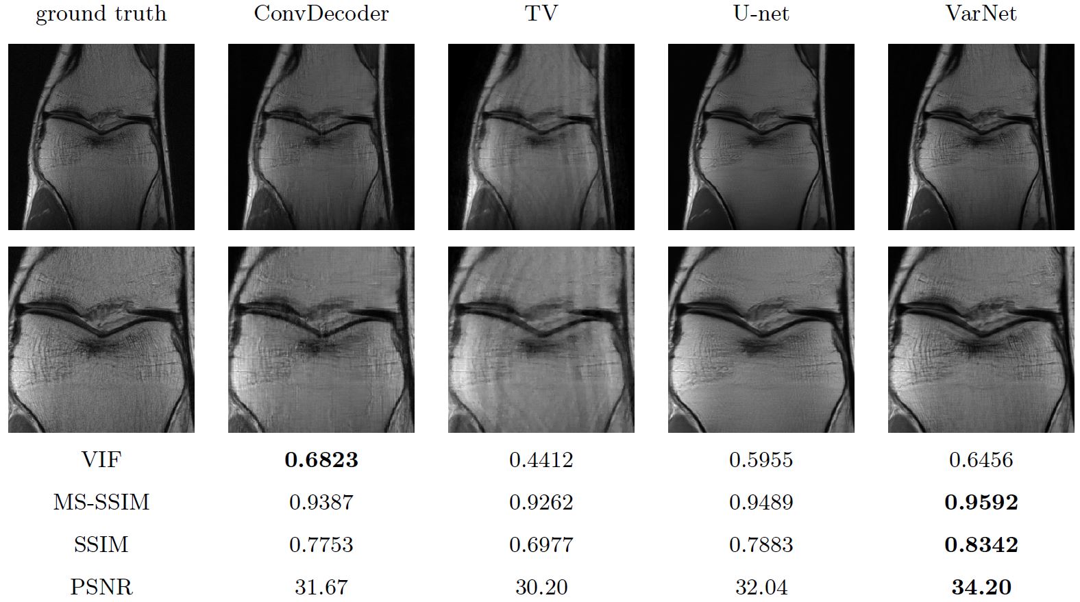
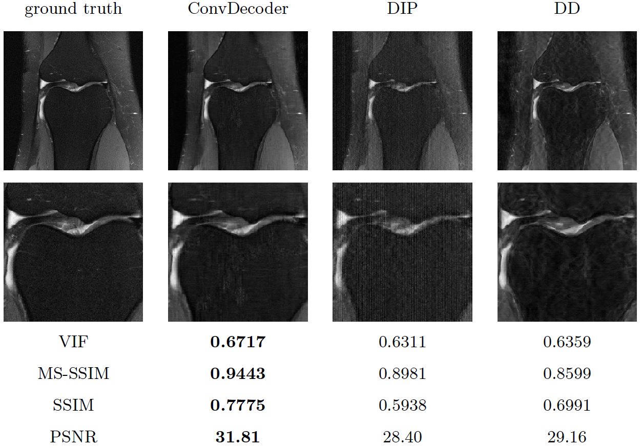
In Figure 2, we show the reconstruction results for an example image, as well as the Visual Information Fidelity (VIF), Multi-Scale SSIM (MS-SSIM), SSIM, and PSNR scores averaged over 200 center slices of the knee FastMRI10 dataset. The VIF score is considered to be most aligned with radiologists' evaluations of images11. The results show that the ConvDecoder without training performs as well as a trained U-net and significantly better than a conventional sparsity-based method (TV) for 4x acceleration.Figure 3 compares the performance of the ConvDecoder architecture to the DIP and DD architectures. All architectures use our data-consistency step. The results show that the data-consistency step proposed here improves the results for all methods, and that the ConvDecoder architecture addresses the smoothness and artifacts issues of DIP and DD.
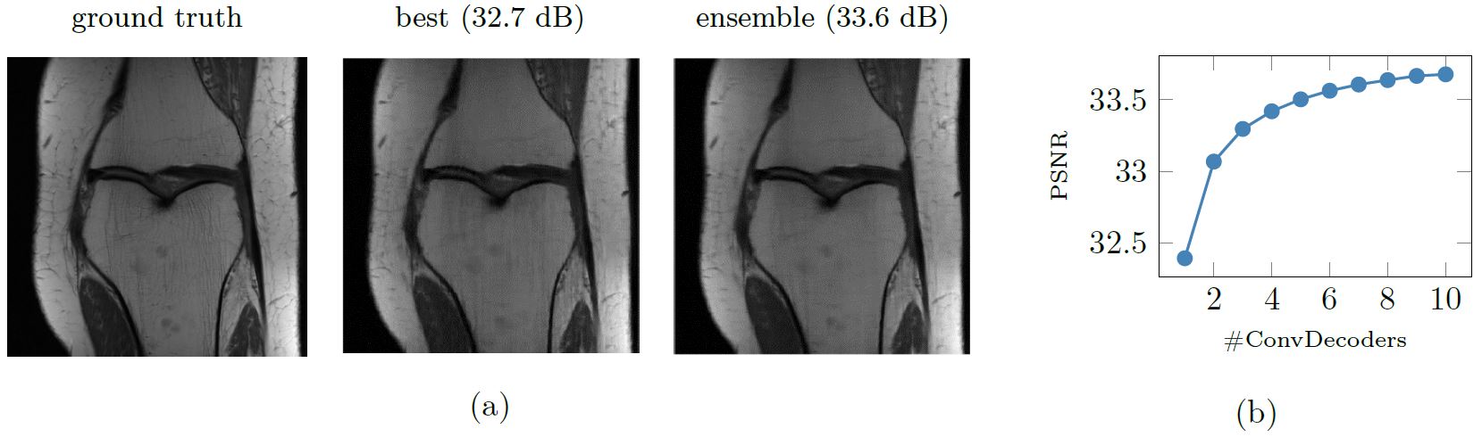
Figure 4 shows that our ensembling technique enhances the reconstruction quality and also demonstrates how PSNR score changes by varying the number of considered decoders.
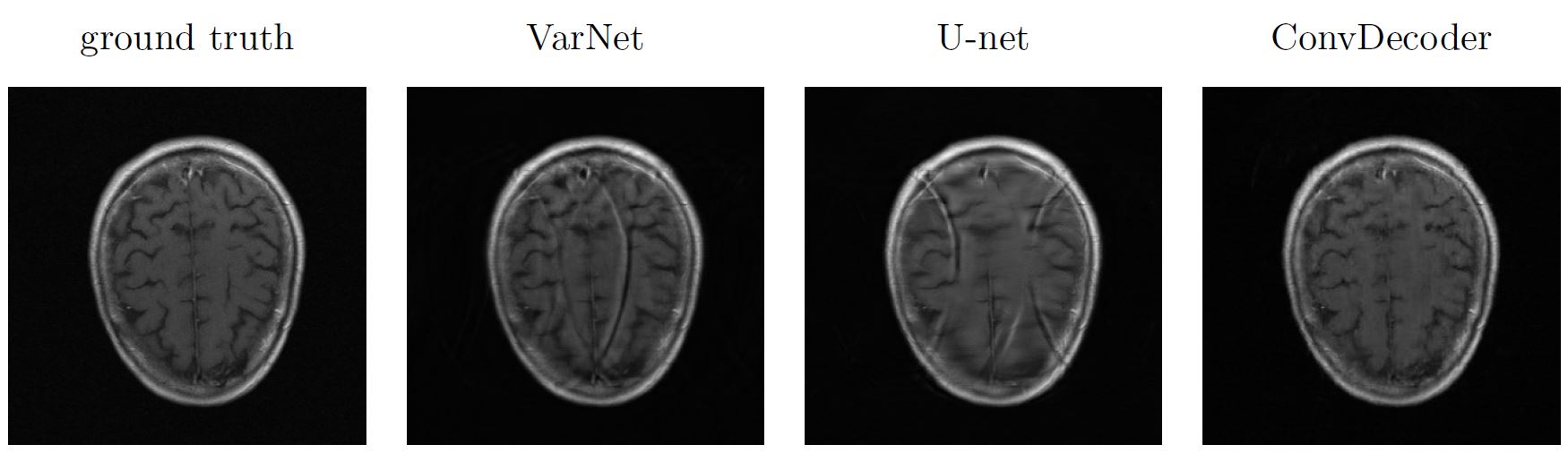
Finally, Figure 5 illustrates that for an out-of-distribution example (i.e., a brain image for networks trained on knees), trained neural networks lose significant performance, whereas un-trained networks are by design robust to such shifts.
The code to reproduce our results is available at https://github.com/MLI-lab/ConvDecoder, and the full version of this paper is available as a preprint on arXiv12.
Discussion and Conclusion
This work shows that, perhaps surprisingly, an un-trained network (i) can achieve similar performance to a baseline trained network and only performs slightly worse than the state-of-the-art trained methods, and it (ii) by design generalizes better to out-of-distribution examples. We achieved this performance through architectural and algorithmic improvements.While the state-of-the-art trained neural networks still slightly outperform our un-trained network in terms of reconstruction accuracy, (i) the robustness to distribution shifts and (ii) not needing any training data make un-trained networks an important tool in practice, especially in regimes where there is a lack of training data, and a need for robustness.
Acknowledgements
R. Heckel and M. Zalbagi Darestani are partially supported by NSF award IIS-1816986, and R. Heckel acknowledges support of the NVIDIA Corporation in form of a GPU, and is partially supported by the IAS at TUM. The authors would like to thank Zalan Fabian for sharing his finding that averaging the outputs of multiple runs of deep decoders improves denoising performance, which led us to study the performance of averaging multiple ConvDecoder outputs (i.e., Figure 4). The authors would also like to thank Lena Heidemann for helpful discussions and for running a grid search on the brain images for the Deep Decoder.References
1. A. Sriram et al. “End-to-end variational networks for accelerated MRI reconstruction”. In: arXiv:2004.06688 [eess.IV]. 2020.
2. O. Ronneberger, P. Fischer, and T. Brox. “U-net: convolutional networks for biomedical image segmentation”. In: International Conference on Medical Image Computing and Computer-Assisted Intervention. 2015, pp. 234–241.
3. D. Ulyanov, A. Vedaldi, and V. Lempitsky. “Deep image prior”. In: IEEE Conference on Computer Vision and Pattern Recognition. 2018, pp. 9446–9454.
4. R. Heckel and P. Hand. “Deep Decoder: concise image representations from untrained nonconvolutional networks”. In: International Conference on Learning Representations (ICLR). 2019.
5. D. V. Veen, A. Jalal, M. Soltanolkotabi, E. Price, S. Vishwanath, and A. G. Dimakis. “Compressed sensing with deep image prior and learned regularization”. In: arXiv:1806.06438 [stat.ML]. 2018.
6. S. Arora, V. Roeloffs, and M. Lustig. “Untrained modified deep decoder for joint denoising parallel imaging reconstruction”. In: International Society for Magnetic Resonance in Medicine Annual Meeting. 2020.
7. D. P. Kingma and J. Ba. “Adam: a method for stochastic optimization”. In: International Conference on Learning Representations (ICLR). 2015.
8. M. Uecker et al. “ESPIRiT—an eigenvalue approach to autocalibrating parallel MRI: where SENSE meets GRAPPA”. In: 2014, pp. 990–1001.
9. K. T. Block, M. Uecker, and J. Frahm. “Undersampled radial MRI with multiple coils. Iterative image reconstruction using a total variation constraint”. In: Magnetic Resonance in Medicine: An Official Journal of the International Society for Magnetic Resonance in Medicine. 2007, pp. 1086–1098.
10. J. Zbontar et al. “FastMRI: An open dataset and benchmarks for accelerated MRI”. In: arXiv:1811.08839 [cs.CV]. 2018.
11. A. Mason et al. “Comparison of objective image quality metrics to expert radiologists’ scoring of diagnostic quality of MR images”. In: IEEE Transactions on Medical Imaging. 2019, pp. 1064–1072.
12. M. Z. Darestani and R. Heckel. “Can Un-trained Neural Networks Compete with Trained Neural Networks at Image Reconstruction?” In: arXiv preprint:2007.02471[eess.IV]. 2020.
Figures