0066
Coil Sketching for fast and memory-efficient iterative reconstruction1Department of Bioengineering, Stanford University, Stanford, CA, United States, 2Department of Radiology, Stanford University, Stanford, CA, United States, 3Department of Electrical Engineering, Stanford University, Stanford, CA, United States, 4Cardiovascular Institute, Stanford, CA, United States
Synopsis
Parallel imaging and compressed sensing reconstruction of large datasets has a high computational cost, especially for 3D non-Cartesian acquisitions. This work is motivated by the success of iterative Hessian sketching methods in machine learning. Herein, we develop Coil Sketching to lower computational burden by effectively reducing the number of coils actively used during iterative reconstruction. Tested with 2D radial and 3D cones acquisitions, our method yields considerably faster reconstructions (around 2x) with virtually no penalty on reconstruction accuracy.
Introduction
Parallel imaging and compressed sensing (PICS) reconstruction can substantially reduce acquisition times.1-3 However, long computation time in iterative reconstruction remains a bottleneck for clinical deployment, especially in 3D non-Cartesian acquisitions.A general approach to decrease computation time is to reduce the number of coils actively used during reconstruction. One class of methods is coil compression4-7(CC) which linearly combines multi-channel data prior to reconstruction. While effective for Cartesian imaging, coil compression inherently loses signal energy, which often results in shading artifacts for non-Cartesian imaging. Another approach8,9 uses the stochastic gradient method, which randomly selects subsets of coil channels for each iteration in reconstruction. While fully leveraging all data, it often requires many iterations for convergence.
We propose a reconstruction method, denoted Coil Sketching, that combines the best of both approaches. Our method is based on iterative Hessian sketching (IHS)10 algorithms, which were recently proposed to obtain accurate solutions for large-scale machine learning.10,11 The basic idea is to iteratively use a randomly generated sketching matrix to project the problem onto a low dimensional space. Then, the smaller problem can be solved faster and with small memory footprint. To adapt to MR reconstruction, we design a structured sketching matrix that preserves the Fourier structure and leverages previous work on coil compression. Tested with 2D radial and 3D cones acquisitions, our method yields considerably faster reconstructions with virtually no penalty on reconstruction accuracy.
Theory
PICS reconstructionThe general PICS reconstruction problem is:
$$ x^*= \text{argmin}_x \; f(x) := ||Ax-k||^2_2 + \lambda || Wx ||_1 \; \text{[Eq. 1]}$$
where $$$x$$$ represents the image, $$$A$$$ models the MR imaging process, $$$k$$$ is the acquired k-space, and $$$W$$$ is a sparsifying transform. Matrix $$$A$$$ has the following structure:
$$ A=UFC \; \text{[Eq. 2]}$$
where $$$C$$$ represents the voxel-wise multiplication by $$$c$$$ coil sensitivity maps, $$$F$$$ is the coil-wise FFT, and $$$U$$$ is the undersampling operator. The computational cost of solving Eq. 1 is linearly proportional to the number of coils $$$c$$$.
Iterative Hessian Sketching
When applying IHS algorithms,10,11 we do not solve directly Eq. 1. Instead, we iterate solving lower-dimensional versions with sketched model matrices $$$A^t_S=S^tA$$$, where $$$S^t$$$ is the randomly generated sketching matrix at iteration $$$t$$$ . For L1-regularized problems, at each iteration, the next estimate $$$x^t$$$ is:
$$x^{t+1} = \text{argmin}_x \; \hat{f}(x) := || A^t_S(x - x^t) ||^2_2 - x^TA^T(k - Ax^t) + \lambda || Wx ||_1 \; \text{[Eq. 3]}$$
Structured sketching matrix S
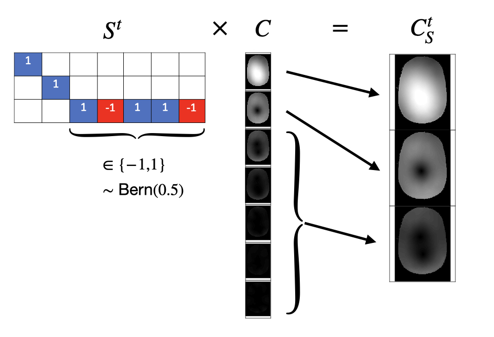
We propose a structured sketching matrix $$$S$$$, denoted Eigen-Sketching matrix, that effectively reduces the number of coils in the model matrix A. Similar to CC,4-7 this matrix considers the high-energy virtual coils, which are extracted from principal components of multi-channel k-space. But unlike CC, the matrix also considers random linear combinations of the remaining low-energy coils. Fig. 1 provides an illustration. This design has two main features: (1) the matrix preserves the Fourier structure and (2) it is adaptive to multi-channel signal energy.
Concretely, multiplication by the proposed Eigen-Sketching matrix $$$S^t$$$ equivalently performs random linear combinations in the coil dimension. As $$$U$$$ and $$$F$$$ are coil-wise linear operations, sketching $$$A$$$ will be equivalent to directly sketching matrix $$$C$$$, which yields a $$$C^t_S$$$ operator with a reduced number $$$\hat{c} < c$$$ of sensitivity maps:
$$A^t_S = S^t = S^t (UFC) = UFC^t_S \; \text{[Eq. 4]}$$
Methods
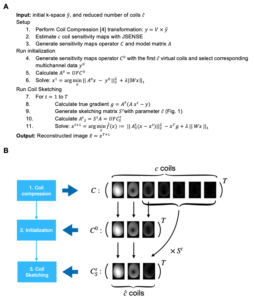
Algorithm pipelineFig. 2 presents the algorithm pipeline. We empirically selected the number of virtual coils $$$\hat{c} < c$$$ that accumulated at least 80% of the total energy. First, to accelerate convergence, we perform an initialization that runs with the first $$$\hat{c}$$$ virtual coils. This process yields a fast yet inaccurate first estimate of $$$x$$$. Then, we apply our proposed Coil Sketching scheme to iteratively refine $$$x$$$. At each iteration, we calculate $$$A^t_s$$$, and solve Eq. 3. Both reconstructions with coil compression and Coil Sketching use model matrices that effectively work with $$$\hat{c}$$$ coils. Thus, the computational cost is linearly proportional to $$$\hat{c}$$$ instead of the number of coils $$$c$$$.
Evaluation
We tested our method with two retrospectively $$$R=2$$$ undersampled datasets:
- Liver 2D radial acquisition with tiny golden angle, 32 channel cardiac coil, $$$256/512$$$ readouts, image size (256x256)
- Abdominal 3D cones acquisition, 20 phases array torso coil, $$$21136/42272$$$ readouts, image size (297x297x112)
- Reconstruction with all coils
- Reconstruction with coil compression using only the first $$$\hat{c}$$$ virtual coils
- Coil Sketching with $$$\hat{c}$$$ coils ( $$$(\hat{c} - 1)$$$ virtual coils and 1 sketched coil)
Results
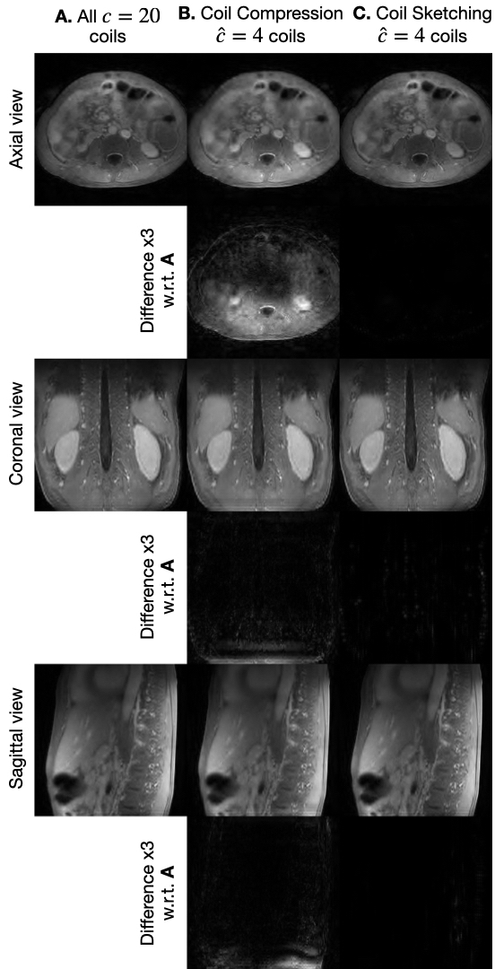
Reconstructions with coil compression and Coil Sketching run considerably faster ($$$\approx 2$$$x) than reconstruction using all coils (Fig. 3). However, reconstruction with coil compression converges to a suboptimal value, whereas the proposed method attains the optimal value. This suboptimality is manifested as significant lower image quality (Fig. 4) and noticeable shading artifacts in the 3D acquisition (Fig. 5).Conclusion & Discussion
Coil Sketching allows faster reconstruction and improved memory-efficiency, by effectively using fewer sensitivity maps and, therefore, less Fourier transform per iteration. This reduced computational cost could enable reconstruction of larger datasets with higher resolution and dimensionality.Acknowledgements
This project was supported by NIH R01 EB026136 and NIH R01 EB009690.References
1. Lustig, M., Donoho, D. and Pauly, J.M., 2007. Sparse MRI: The application of compressed sensing for rapid MR imaging. Magnetic Resonance in Medicine: An Official Journal of the International Society for Magnetic Resonance in Medicine, 58(6), pp.1182-1195.
2. King, K.F., 2008. Combining compressed sensing and parallel imaging. In Proceedings of the 16th annual meeting of ISMRM, Toronto (Vol. 1488, p. 44).
3. Vasanawala, S.S., Murphy, M.J., Alley, M.T., Lai, P., Keutzer, K., Pauly, J.M. and Lustig, M., 2011, March. Practical parallel imaging compressed sensing MRI: Summary of two years of experience in accelerating body MRI of pediatric patients. In 2011 IEEE international symposium on biomedical imaging: From nano to macro (pp. 1039-1043). IEEE.
4. Zhang, T., Pauly, J.M., Vasanawala, S.S. and Lustig, M., 2013. Coil compression for accelerated imaging with Cartesian sampling. Magnetic resonance in medicine, 69(2), pp.571-582.
5. Buehrer M, Pruessmann K, Boesiger P, Kozerke S. Array compression for MRI with large coil arrays. Magn Reson Med 2007;57:1131–1139.
6. Huang F, Vijayakumar S, Li Y, Hertel S, Duensing G. A software channel compression technique for faster reconstruction with many channels. Magn Reson Imaging 2008;26:133–141.
7. King S, Varosi S, Duensing G. Optimum SNR data compression in hardware using an eigencoil array. Magn Reson Med 2010;63:1346–1356.8.
8. Muckley MJ, Noll DC, Fessler JA. Accelerating SENSE-type MR image reconstruction algorithms with incremental gradients. In: Proceedings of the ISMRM 22nd Annual Meeting, Milan, Italy; March 2014:4400.9.
9. Ong, F., Zhu, X., Cheng, J.Y., Johnson, K.M., Larson, P.E., Vasanawala, S.S. and Lustig, M., 2020. Extreme MRI: Large‐scale volumetric dynamic imaging from continuous non‐gated acquisitions. Magnetic Resonance in Medicine.
10. Pilanci, M. and Wainwright, M. J. Iterative hessian sketch: Fast and accurate solution approximation for constrained least-squares. Journal of Machine Learning Research, 17(53):1–38, 2016.
11. Tang, J., Golbabaee, M. and Davies, M.E., 2017, July. Gradient projection iterative sketch for large-scale constrained least-squares. In International Conference on Machine Learning (pp. 3377-3386). PMLR.
12.Charikar, M., Chen, K. and Farach-Colton, M., 2004. Finding frequent items in data streams. Theoretical Computer Science, 312(1), pp.3-15.
13. Clarkson, K.L. and Woodruff, D.P., 2017. Low-rank approximation and regression in input sparsity time. Journal of the ACM (JACM), 63(6), pp.1-45.
14. Pham, N. and Pagh, R., 2013, August. Fast and scalable polynomial kernels via explicit feature maps. In Proceedings of the 19th ACM SIGKDD international conference on Knowledge discovery and data mining (pp. 239-247).
15. Ying, L., & Sheng, J. (2007). Joint image reconstruction and sensitivity estimation in SENSE (JSENSE). Magnetic Resonance in Medicine, 57(6), 1196-1202.
Figures